An integrated and cooperative architecture for multi-intersection traffic signal control

Qiang Wu; Jianqing Wu; Bojian Kang; Bo Du; Jun Shen; Adriana Simona Mihăiţă; Qiang Wu; Jianqing Wu; Bojian Kang; Bo Du; Jun Shen; Adriana Simona Mihăiţă

doi:10.48130/DTS-2023-0012

Figures (12) Tables (10)

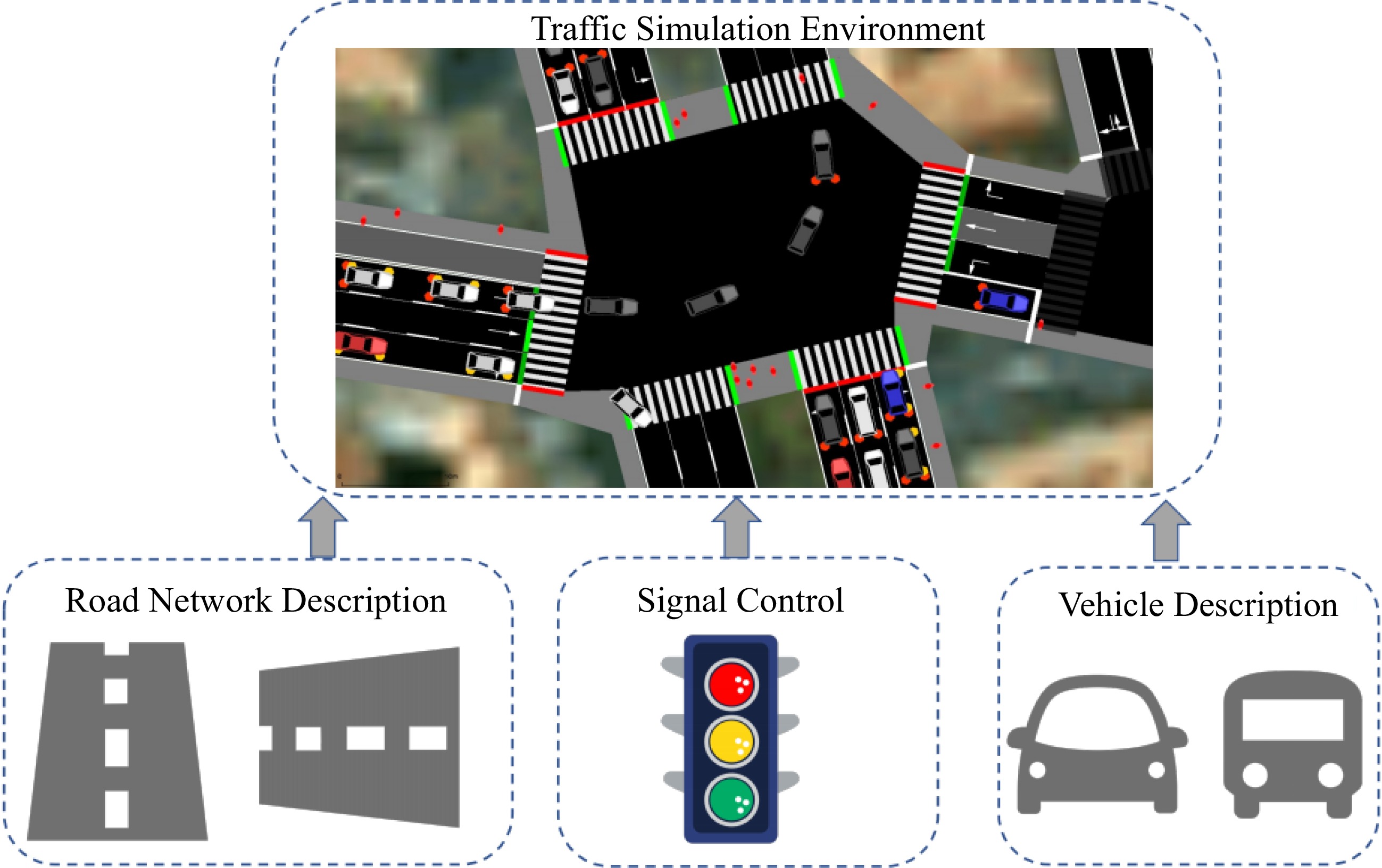
Figure 1.
An urban traffic simulation environment for traffic research.
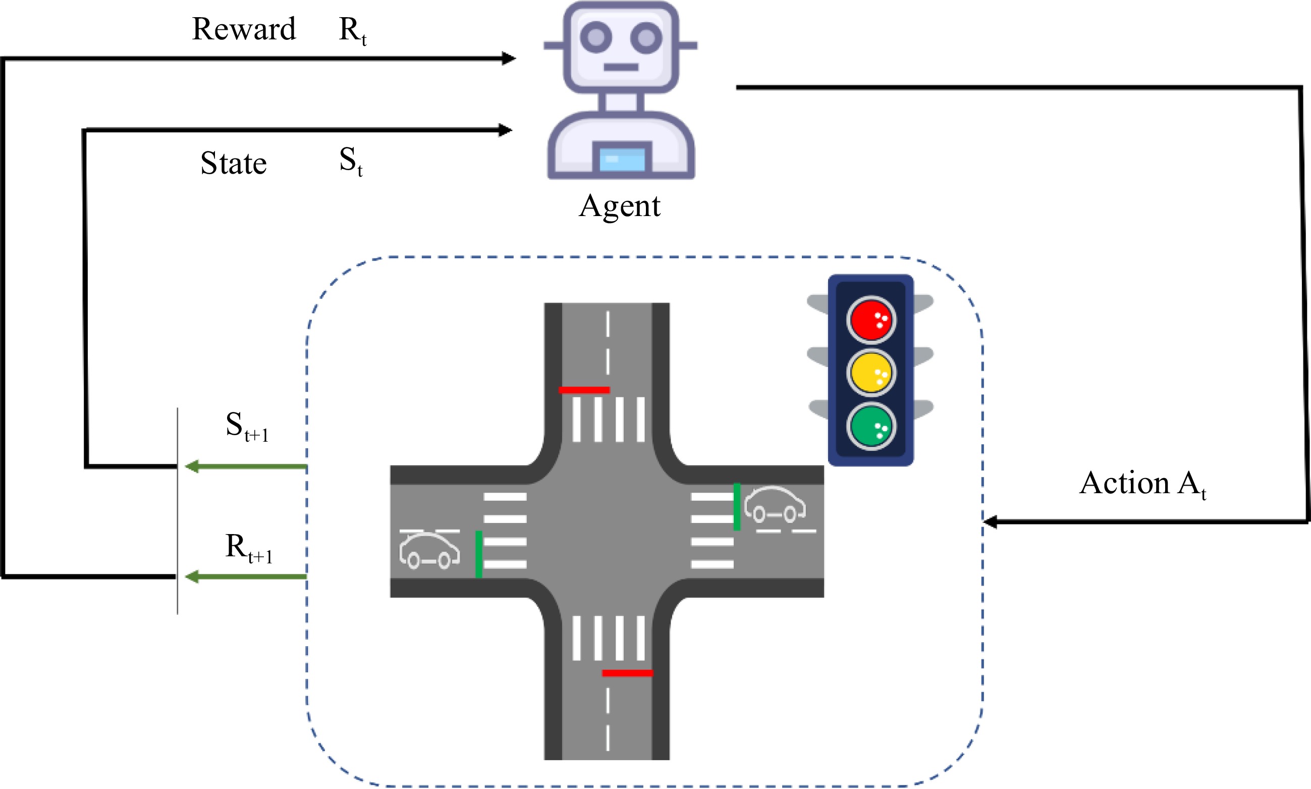
Figure 2.
An illustration of traffic signal control at an intersection. According to the current traffic state $ {S}_{t} $ and the reward $ {R}_{t} $, the agent selects and executes the corresponding action $ {A}_{t} $ (change or maintain the current traffic light). Then the agent evaluates the effects of the action to obtain a new traffic state $ {S}_{t+l} $ and a new reward $ {R}_{t+1} $.
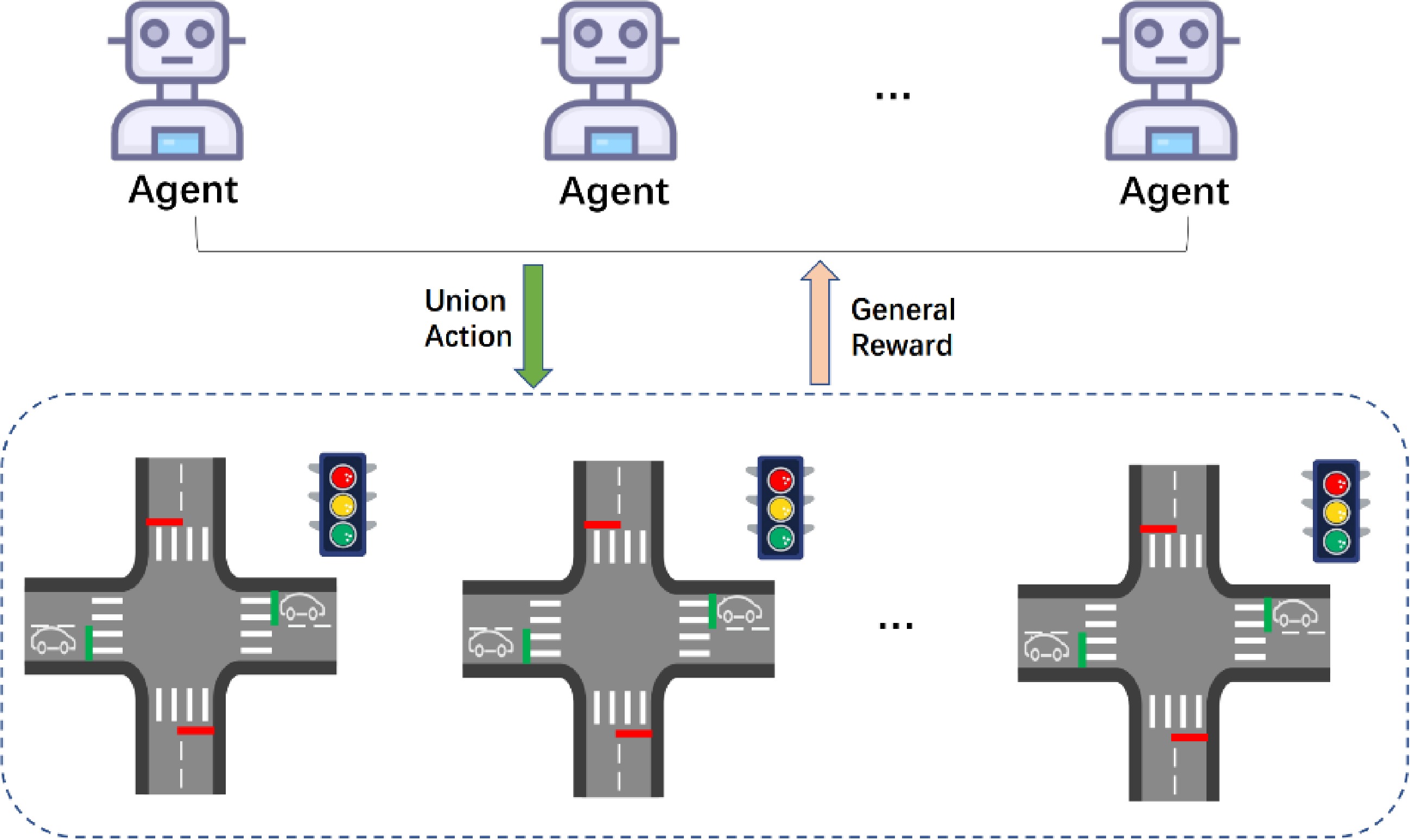
Figure 3.
The MARL structure in urban traffic signal control.
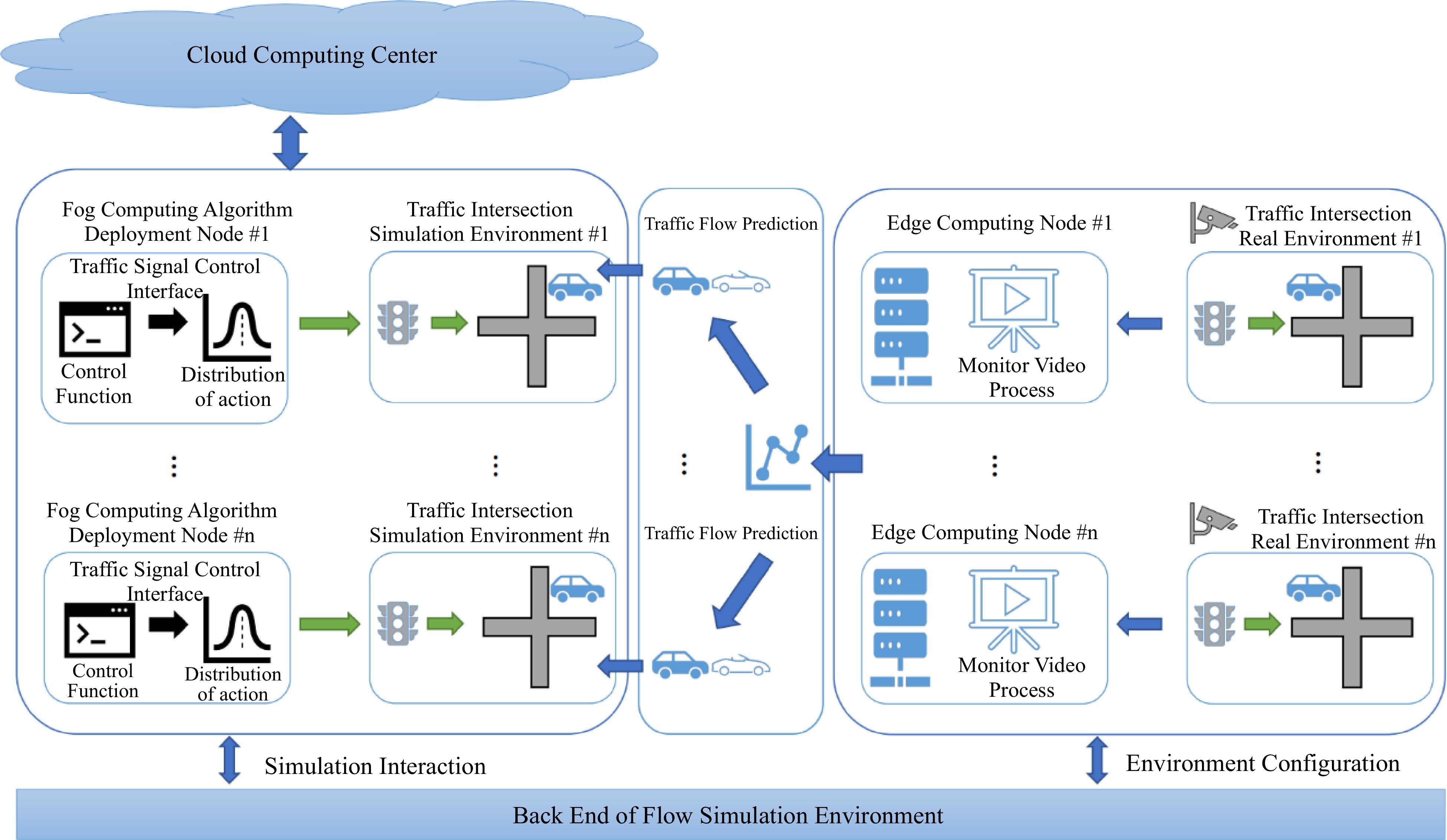
Figure 4.
The General City Traffic Computing System (GCTCS) for urban traffic signal control.
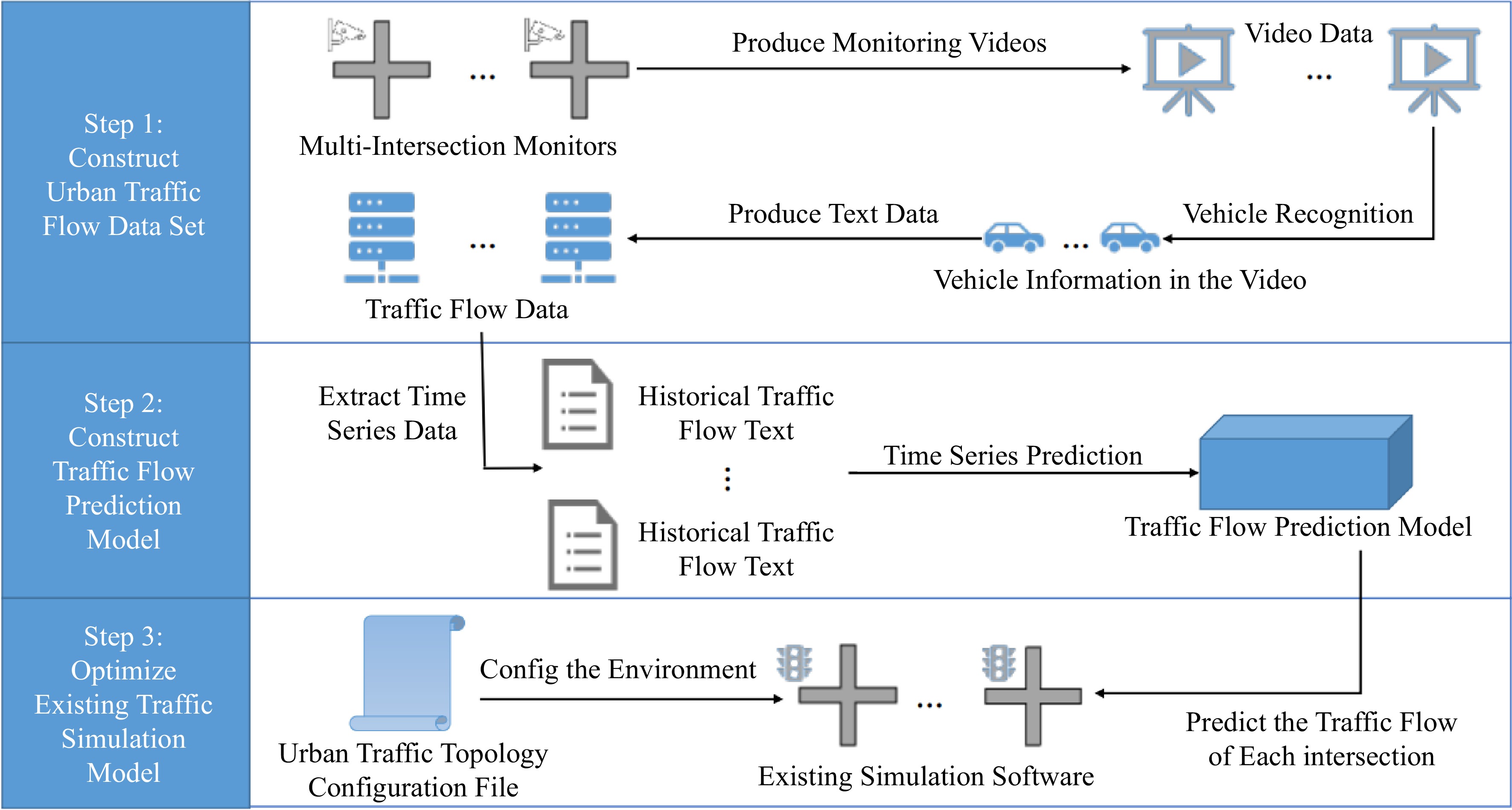
Figure 5.
The processes of construction of the urban traffic real environment.
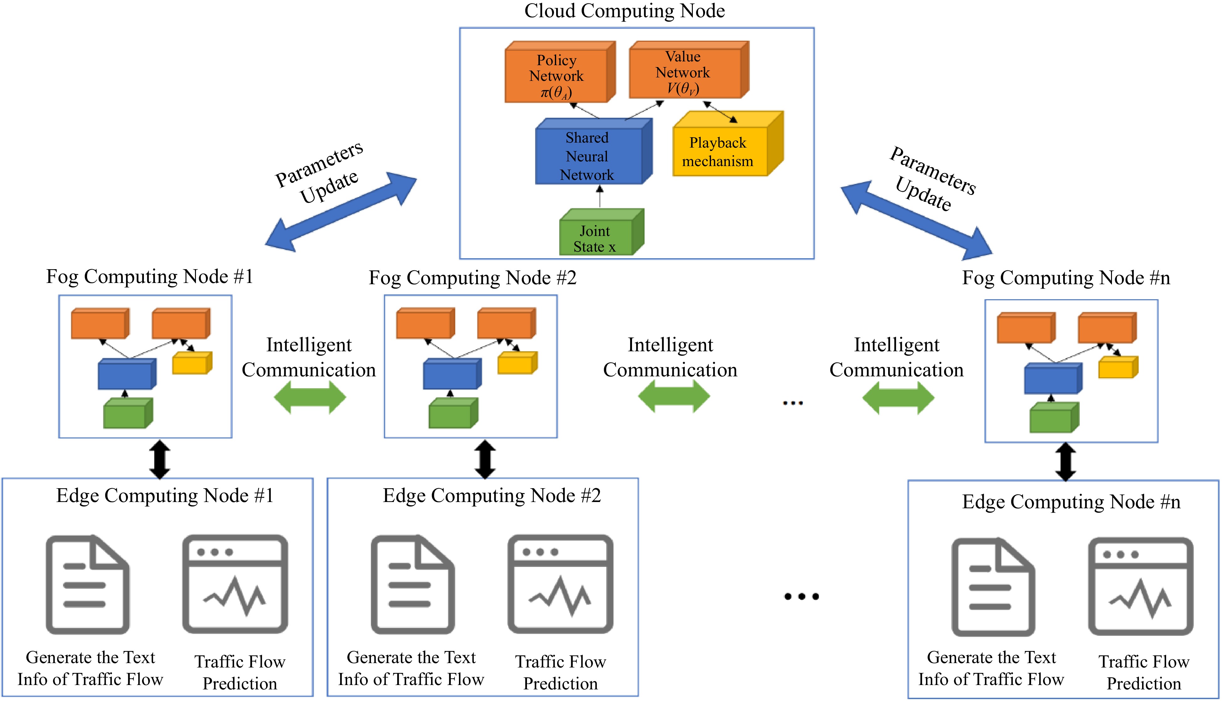
Figure 6.
The General-MARL is composed of three sub-algorithms based on different layers of the GCTCS architecture.
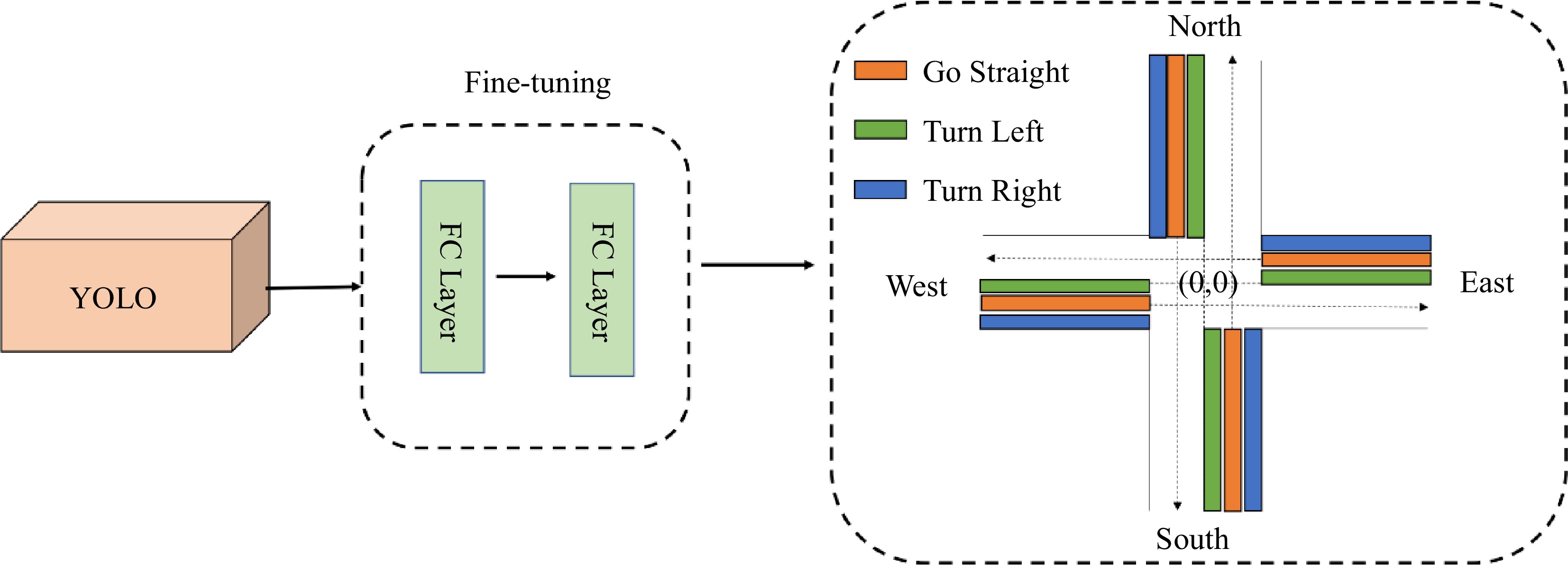
Figure 7.
The process of abstracting traffic information from the video to generate the text info from traffic flow. Detection of vehicles in the three regions stands for different directions of passing vehicles
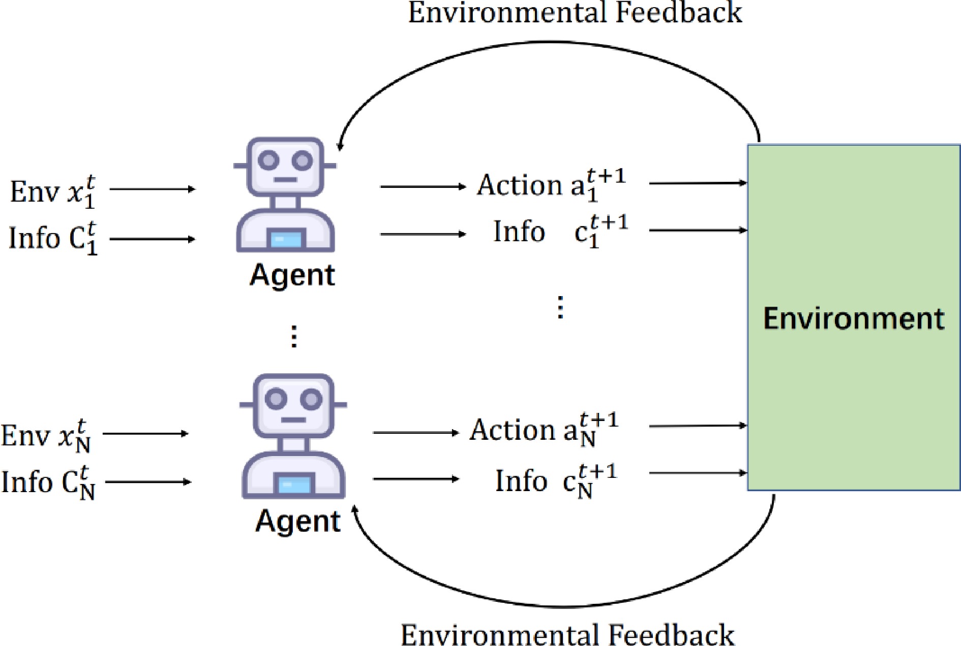
Figure 8.
The communication process between agents in the communication module.
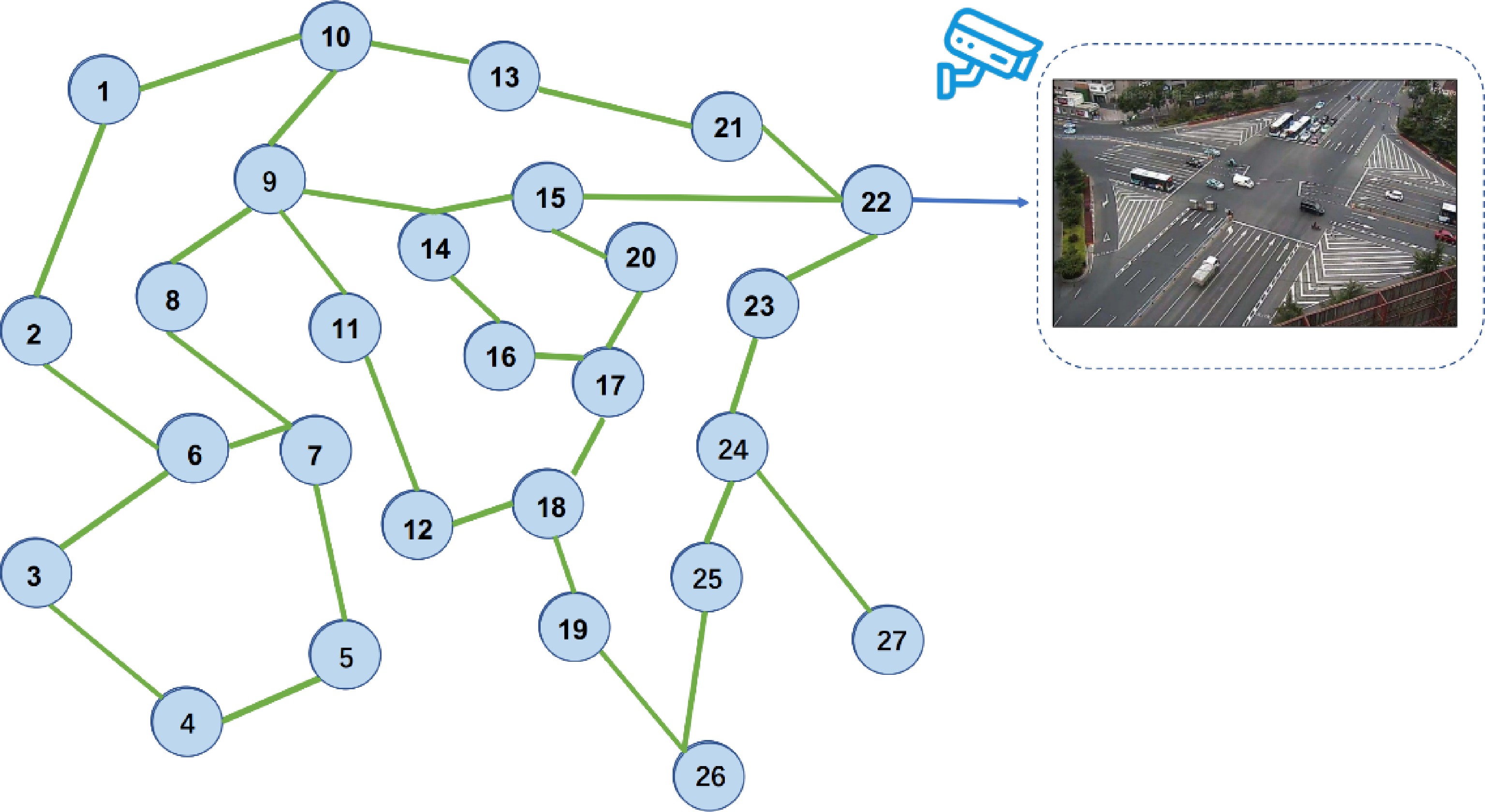
Figure 9.
The illustration of topology map of real traffic intersection.
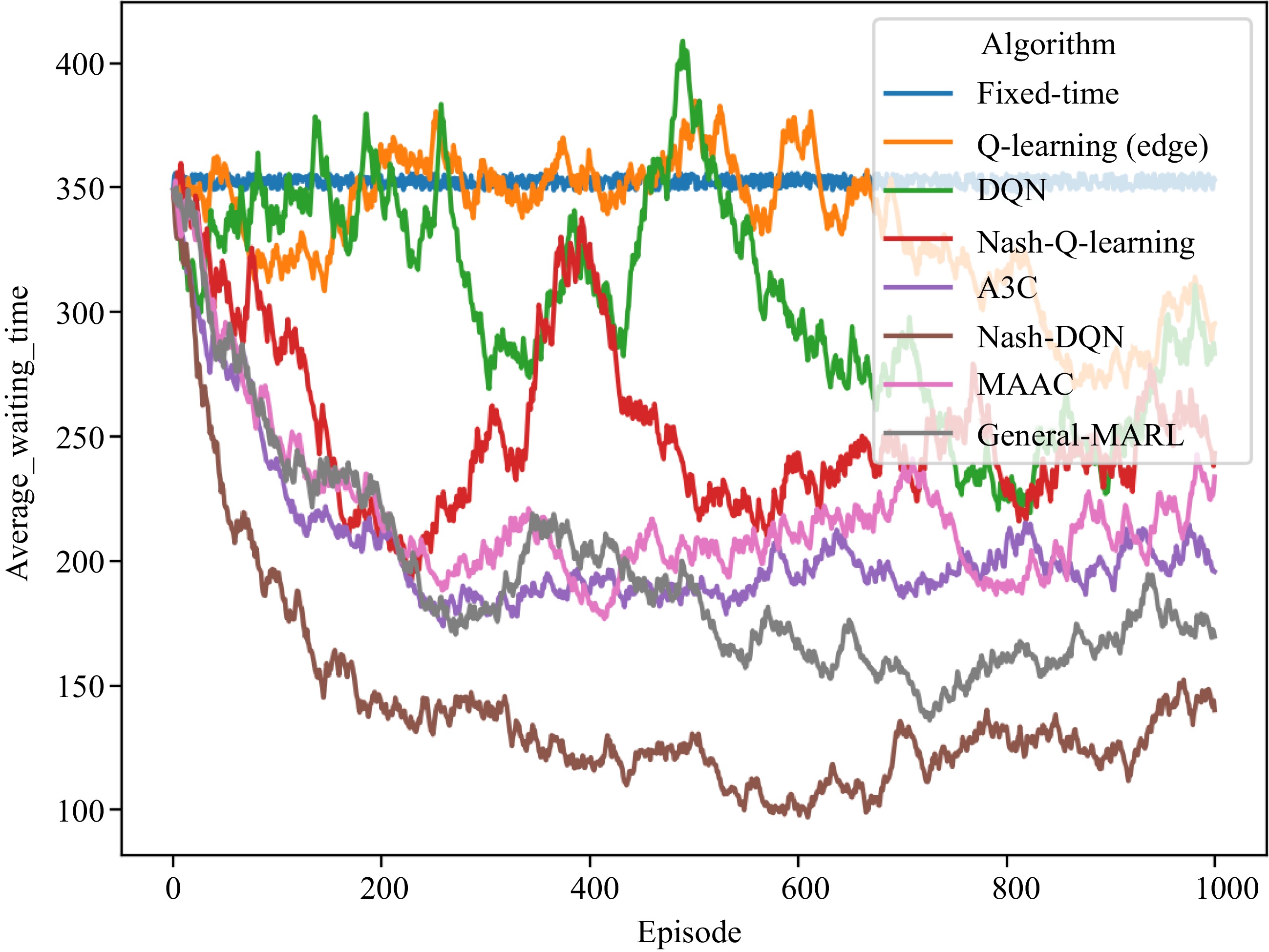
Figure 10.
Multi-intersection traffic signal control training process (without network delay).
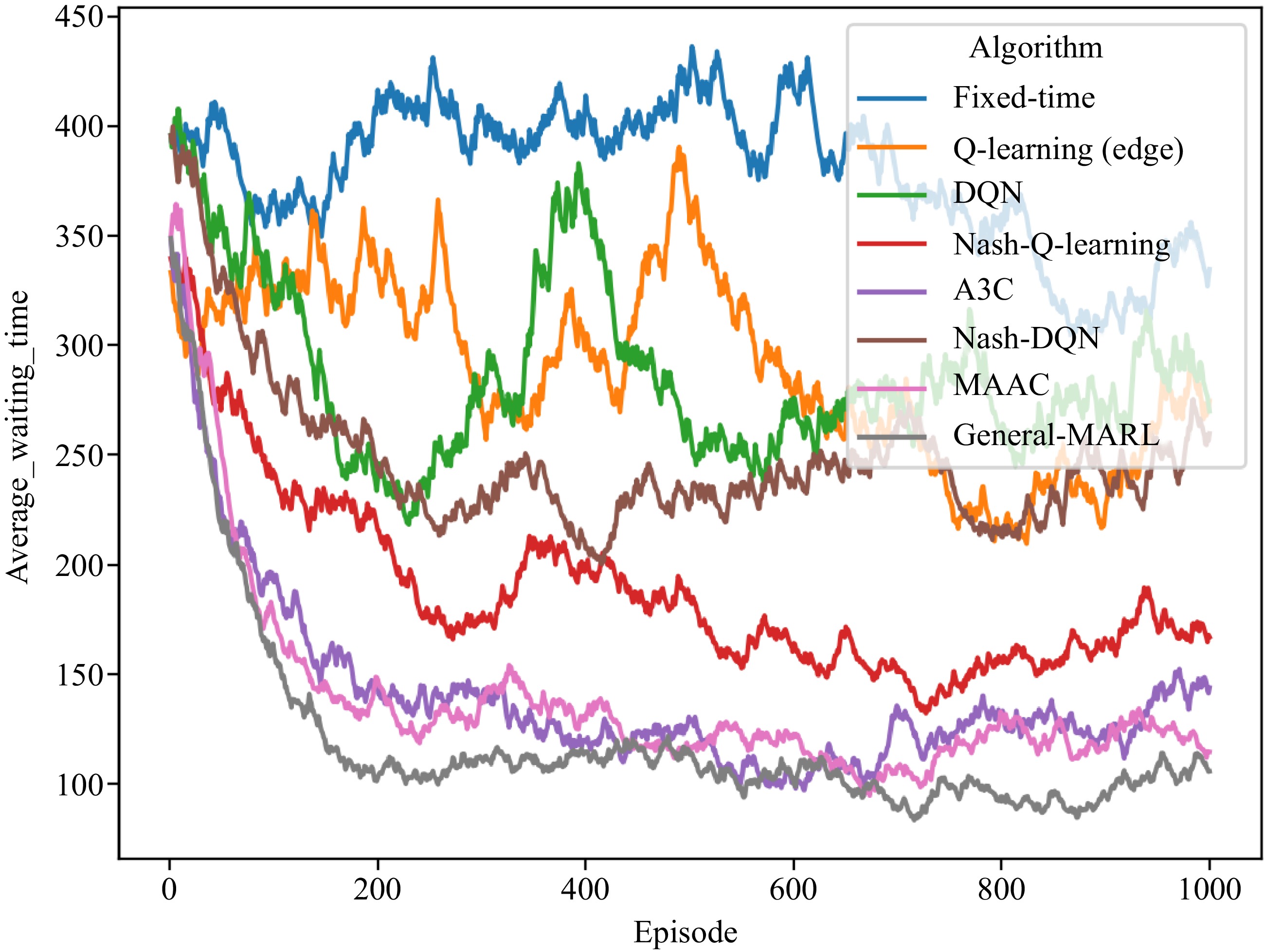
Figure 11.
Multi-intersection traffic signal control training process (with network delay).
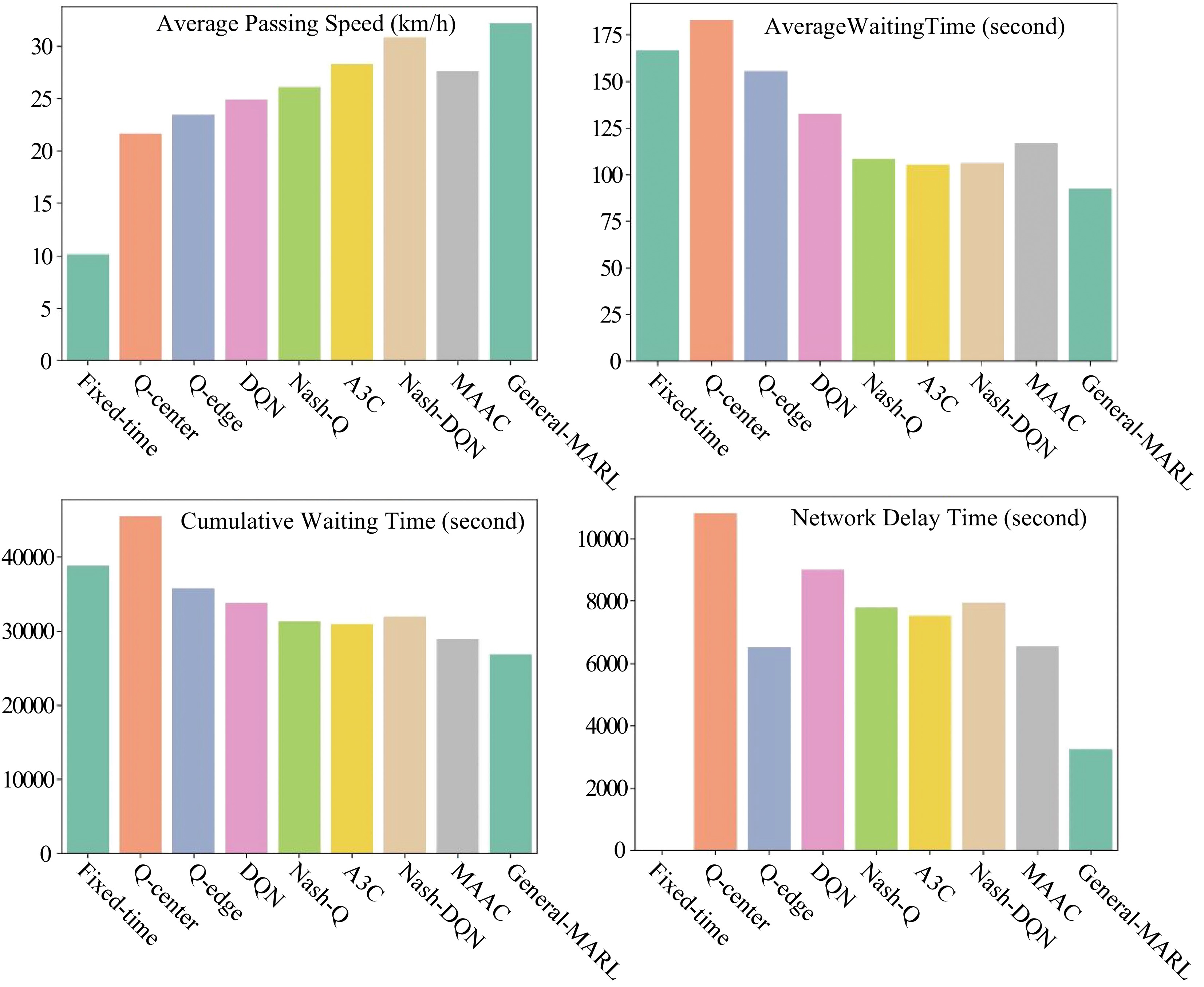
Figure 12.
Comparative results among different algorithms.

1: Input the video information of the traffic situation.

2: Capture one frame from the video: G

3: Use and fine-tune the YOLO to recognize all the vehicle's position (x,y) and type in G.

4: for vehicle in G do

5: Obtain the direction of vehicles by judging the (x,y) from the regions according the three regions predefined.

6: Record traffic state text information (vehicle -id, types, direction, and the timestamp) into traffic state text T.

7: end for

8: Use GCN-GAN for traffic flow prediction to T.

9: Connect traffic flow prediction capability to the urban simulation environment.

Table 1.

Edge-General-control algorithm.

1:	Init Episode $ B > 0 $, $ b=1 $; Minibatch Size $ \hat{M} > 0 $, Game Step N
2:	Init Replay Buffer $ D $, $ {\theta }_{V} $ and $ {\theta }_{A} $
3:	repeat
4:	Reset, go to the $ {x}_{0} $
5:	repeat
6:	Select $ u\leftarrow {\pi }^{{\theta }_{A}}\left(x\right) $ or select $ u $ randomly (e.g., ϵ-greedy)
7:	Observe $ {y}_{t}=\left({x}_{t-1},u,{x}_{t}\right) $
8:	Store $ {y}_{t} $ to Reply Buffer $ D $
9:	Sampling from Replay Buffer: $ Y={\left\{{y}_{i}\right\}}_{i=1}^{\hat{M}} $
10:	Optimize $ \frac{1}{M+1}{\sum }_{y\in Y\cup \left\{{y}_{t}\right\}}\hat{L}\left(y,{\theta }_{V},{\theta }_{A}\right) $ fix $ {\theta }_{A} $ update $ {\theta }_{V} $
11:	Optimize $ \frac{1}{M+1}{\sum }_{y\in Y\cup \left\{{y}_{t}\right\}}\hat{L}\left(y,{\theta }_{V},{\theta }_{A}\right) $ fix $ {\theta }_{V} $ update $ {\theta }_{A} $
12:	Until $ t > N $
13:	Until $ b > B $
14:	return $ {\theta }_{V} $ and $ {\theta }_{A} $

Table 2.

Nash-MARL Module.

1: Initialize the communication matrix of all agents

$ {C}_{0} $

2: Initialize the parameters of agent

$ {\theta }_{Sender}^{i} $

and

$ {\theta }_{Receiver}^{i} $

3: repeat

4: Receiver of

$ {Agent}^{i} $

: use attention mechanism to generate communication matric

$ {\hat{C}}_{t} $

5: Sender of

$ {Agent}^{i} $

: chooses an action

$ {a}_{t+1}^{i} $

from policy selection network, or randomly chooses an action (e.g., ϵ-greedy exploration)

6: Sender of

$ {Agent}^{i} $

: generate its own information through the receiver's communication matrix

$ {\hat{C}}_{t}:{c}_{t+1}^{i} $

7: Collect all the joint actions of Agent and execute the actions

$ {a}_{t+1}^{1},\cdots ,{a}_{t+1}^{N} $

, get the reward from the environment

$ {R}_{t+1} $

and next state

$ {X}_{t+1} $

8: until End of Round Episode

9: return

$ {\theta }_{Sender}^{i} $

and

$ {\theta }_{Receiver}^{i} $

for each agent

Table 3.

The communication module.

1: Apply the communication module:
2: Initialize the communication matric $ {C}_{0} $ of all fog computing node Agents
3: Initialize the parameters $ {\theta }_{Sender}^{i} $ and $ {\theta }_{Receiver}^{i} $ of the fog computing node Agents
4: Receive the global parameter sets $ {\theta }_{V} $ and $ {\theta }_{A} $ distributed by the cloud computing node and initialize the parameter sets $ {\theta }_{V}^{i} $ and $ {\theta }_{A}^{i} $
5: Initialize the Episode $ B > 0 $, $ b=1 $; the minimum batch size Minibatch Size $ \stackrel{-}{M} > 0 $, the number of game steps $ N $
6: Apply the Nash-MARL Module:
7: Initialize the memory record Replay Buffer $ D $
8: repeat
9:	Reset the environment and enter the initial state $ {x}_{0} $
10:	repeat
11:	Choose joint action $ u\leftarrow {\pi }^{{\theta }_{A}}\left(x\right) $ or randomly choose joint action $ u $ (e.g., ϵ-greedy exploration)
12:	Observe the state-action-state triplet $ {y}_{t}=\left({x}_{t-1},u,{x}_{t}\right) $
13:	Store triples in the Replay Buffer $ D $
14:	Extract data $ Y={\left\{{y}_{i}\right\}}_{i=1}^{M} $ from the Replay Buffer
15:	$ {Agent}^{i} $ receiver uses Attention mechanism to generate communication matrix $ {\hat{C}}_{t} $
16:	The strategy choice network of the Agent $ {t}^{i} $ sender chooses an action $ {a}_{t+1}^{i} $, or randomly chooses action a (e.g., ϵ-greedy exploration)
17:	The $ {Agent}^{i} $ sender generates its own information $ {c}_{t+1}^{i} $ through the communication matrix $ {\hat{C}}_{t} $ at the receiving end
18:	Collect the joint actions of all Agents, execute an action $ {a}_{t+1}^{i},\cdots ,{a}_{t+1}^{N} $, get rewards $ {R}_{t+1} $ and the next state $ {X}_{t+1} $ from the environment
19:	Optimization step $ \frac{1}{M+1}{\sum }_{y\in Y\cup \left\{{y}_{t}\right\}}\hat{L}\left(y,{\theta }_{V}^{i},{\theta }_{A}^{i},{\hat{C}}_{t}\right) $, fixes $ {\theta }_{A}^{i} $ updates $ {\theta }_{V}^{i} $
20:	Optimization step $ \frac{1}{M+1}{\sum }_{y\in Y\cup \left\{{y}_{t}\right\}}\hat{L}\left(y,{\theta }_{V}^{i},{\theta }_{A}^{i},{\hat{C}}_{t}\right) $, fixes $ {\theta }_{V}^{i} $ updates $ {\theta }_{A}^{i} $
21:	until $ > N $
22: until $ b > B $
23: Return $ {\theta }_{V}^{i} $ and $ {\theta }_{A}^{i} $

Table 4.

Fog-General-control.

1: Apply the Nash-MARL module:

2: Initialize the global parameter sets

$ {\theta }_{V} $

and

$ {\theta }_{A} $

of the cloud computing center and the global counter

$ T $

3: repeat

4: Distributer global parameters to fog computing nodes

$ {\theta }_{V}^{i}={\theta }_{V} $

$ {\theta }_{A}^{i}={\theta }_{A} $

5: repeat

6: Update global parameters

$ {\theta }_{V}={\theta }_{V}+d{\theta }_{V}^{i} $

$ {\theta }_{A}={\theta }_{A}+d{\theta }_{A}^{i} $

7: until all fog computing nodes are traversed and collected

$ T\leftarrow T+1 $

9: until

$ T > {T}_{max} $

Table 5.

Cloud-General-control.

Module	Parameters	Description
Cloud Computing Center	$ x=0\|x=10 $ 20, 60, 60, 20 0.001	The delay from the cloud to the fog node The hidden layers in the network The learning rate
Fog Computing Node	$ x=0\|x=1 $ 20, 60, 60, 20 0.001	The delay from intersection to the fog node The hidden layers in the network The learning rate
Edge Computing Node	$ x=0\|x=1 $	The delay from edge nodes to fog node
Experiment Settings	$ {g}_{t}={r}_{t}=27,{y}_{t}=6 $ 15 E = 1,000 I = 27 l = 0.001 γ = 0.982	The initial intervals of the green, red and yellow The traffic flow prediction period The number of Episodes The number of intersections The learning rate The discount rate

Table 1.

List of parameters in this paper.

Method Average speed (km/h) Average waiting time (s)

Fixed-time 10.17 166.70
Q learning 18.43 135.62
DQN 20.10 112.24
A3C 24.12 90.73
Nash-Q 29.70 70.14
Nash-DQN 33.81 61.21
MAAC 27.39 80.21
General-MARL 31.22 62.87

Table 2.
Results of General-MARL and other algorithms (ignoring network delay).

Method	Average speed (km/h)	Average waiting time (s)
Fixed-time	10.15	166.71
Q learning(center)	21.69	182.75
Q learning(edge)	23.47	155.64
DQN	24.94	132.70
A3C	26.12	108.65
Nash-Q	28.32	105.55
Nash-DQN	30.86	106.37
MAAC	27.61	116.81
General-MARL	30.78	92.48

Table 3.

Results of the average speed and waiting time in each episode (consider network delay).

Method	Accumulated time (s)	Network delay (s)	Delay rate
Fixed-time	38827.5	0.0	0.0%
Q learning(center)	45448.0	10809.7	23.8%
Q learning(edge)	35789.3	6522.9	18.2%
DQN	33789.9	8997.2	26.6%
A3C	31340.4	7792.1	24.9%
Nash-Q	30940.5	7536.9	24.4%
Nash-DQN	31994.6	7937.7	24.8%
MAAC	28940.7	6552.1	22.6%
General-MARL	26912.7	3264.5	12.2%

Table 4.

Results of accumulated time and network delay in each episode (consider network delay).

ID	Fixed- time	Q-edge	DQN	A3C	Nash-Q	Nash- DQN	MAAC	General
1	175.27	161.96	136.93	110.89	109.34	111.21	124.69	96.81
2	188.35	172.68	145.58	116.43	115.88	119.02	130.73	105.46
3	155.28	145.58	123.71	102.43	99.35	99.27	120.99	83.59
4	197.72	180.36	151.78	120.39	120.57	124.61	133.34	111.66
5	155.23	145.54	123.68	102.41	99.32	99.24	116.97	83.56
6	168.97	156.8	132.76	108.22	106.19	107.45	122.26	92.64
7	157.68	147.55	125.30	103.44	100.55	100.7	107.91	85.18
8	161.32	150.53	127.70	104.98	102.37	102.88	119.31	87.58
9	185.23	170.13	143.52	115.11	114.32	109.88	128.53	103.40
10	176.47	162.95	137.72	111.40	109.94	111.92	115.15	97.60
11	161.21	150.44	127.63	104.94	102.31	102.81	119.28	87.51
12	125.96	121.55	104.32	90.01	104.30	81.77	105.69	64.20
13	131.62	126.19	108.06	92.41	87.52	85.15	117.87	67.94
14	169.15	156.95	132.88	108.30	106.28	107.55	122.33	92.76
15	175.52	180.84	152.16	120.64	109.47	124.96	40.06	112.04
16	132.47	126.89	108.62	92.77	87.94	85.65	108.20	68.50
17	164.12	152.83	129.56	87.56	103.77	104.55	113.46	89.44
18	166.87	155.08	131.38	107.33	105.14	106.19	121.45	91.26
19	150.39	141.57	120.48	100.36	96.90	96.35	115.11	80.36
20	177.77	164.01	138.58	111.95	110.59	112.70	125.65	98.46
21	153.63	144.23	122.62	101.73	98.52	98.29	96.35	82.50
22	167.54	155.63	131.82	107.62	105.48	106.59	121.71	91.70
23	177.62	163.89	162.05	157.98	110.52	112.61	139.54	121.93
24	186.84	171.45	144.58	115.79	115.13	118.11	129.15	104.46
25	175.36	162.04	136.99	110.93	109.39	111.26	128.73	96.87
26	175.23	161.93	136.90	110.87	109.32	111.18	124.67	96.78
27	188.35	172.68	145.58	116.43	115.88	119.02	104.64	102.77

Table 5.

Results of average waiting time at each intersection in each episode (considering network delay).

Method	Average speed (km/h)	Average waiting time (s)
Fixed-time	10.17	166.70
Q learning	18.43	135.62
DQN	20.10	112.24
A3C	24.12	90.73
Nash-Q	29.70	70.14
Nash-DQN	33.81	61.21
MAAC	27.39	80.21
General-MARL	31.22	62.87