-
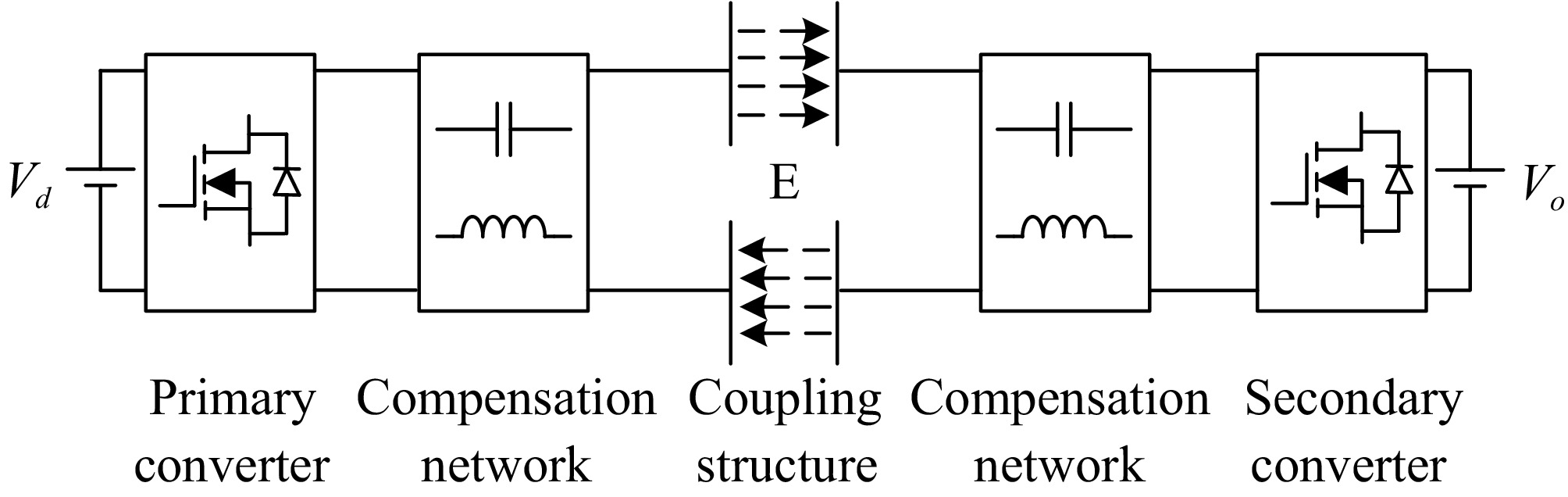
Figure 1.
Block diagram of a typical bidirectional EC-WPT system.
-
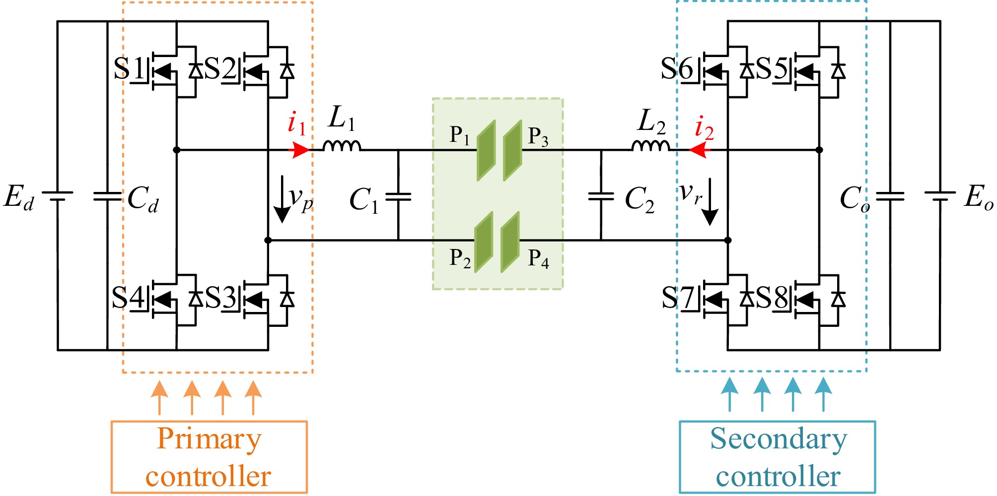
Figure 2.
Circuit topology diagram of the dual LC compensation network bidirectional EC-WPT system.
-
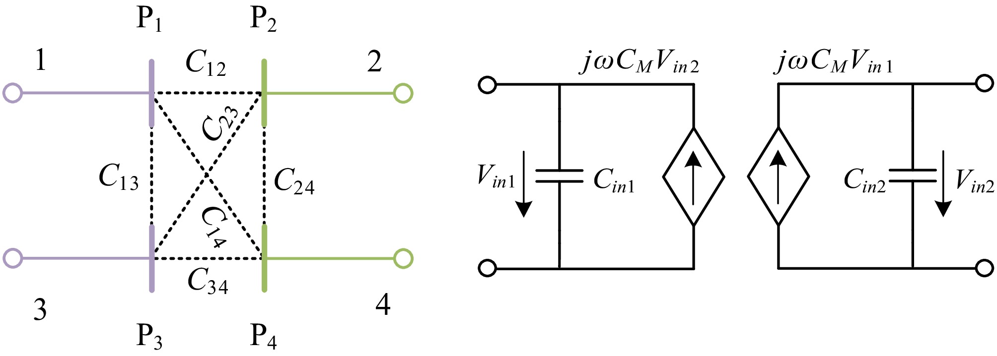
Figure 3.
Equivalent current source model of the coupling structure.
-
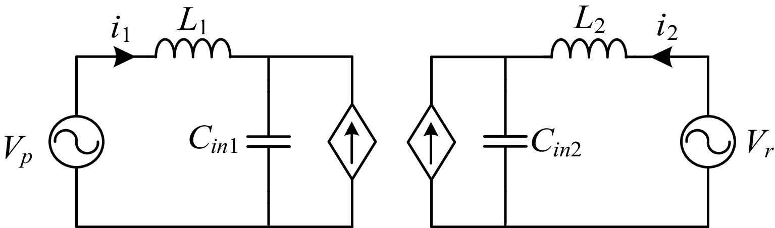
Figure 4.
Equivalent current source circuit model of the bidirectional EC-WPT system.
-
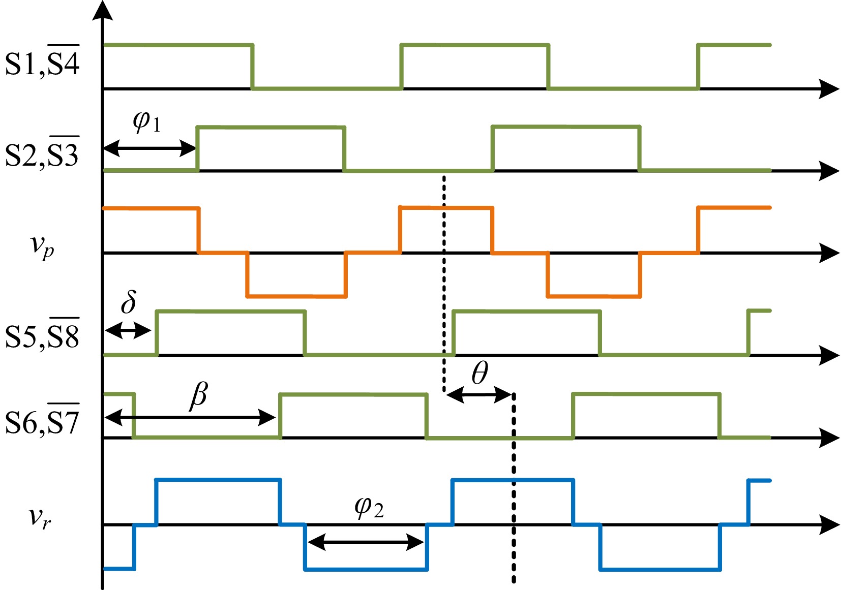
Figure 5.
Switching sequences and resonant voltages of the primary and receiver converters.
-
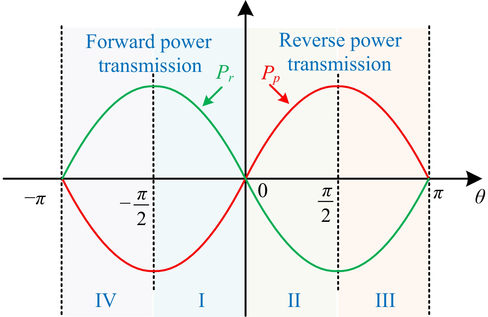
Figure 6.
Phase relationship between transmission power and relative phase angle.
-
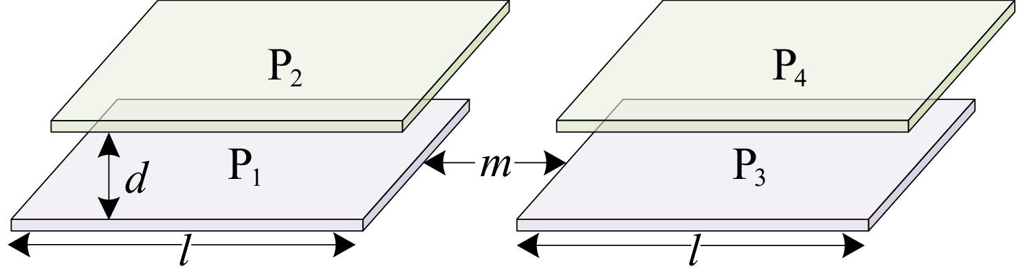
Figure 7.
Structure and dimension of coupling plates.
-
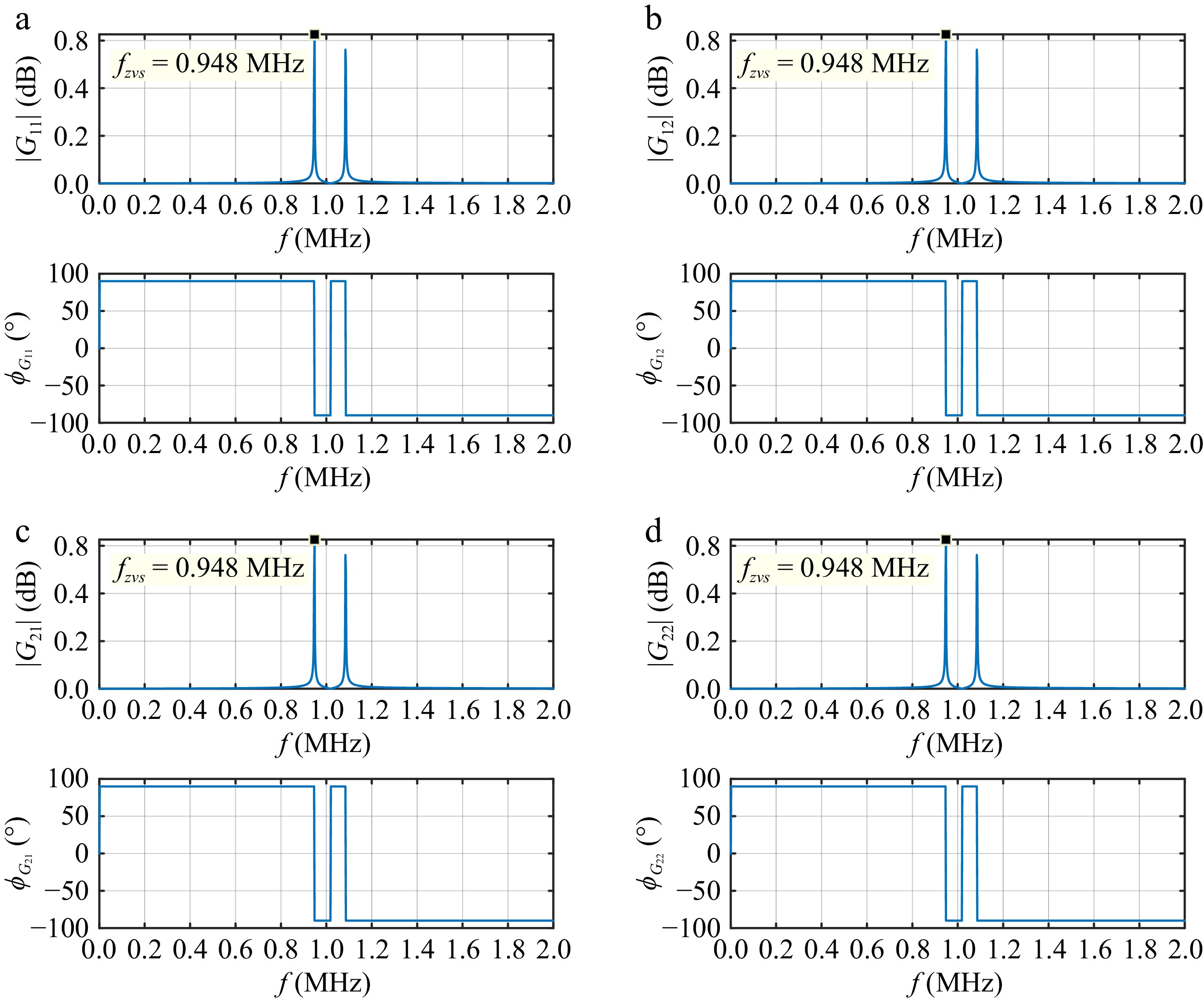
Figure 8.
The magnitude-frequency and phase-frequency curves of the system transfer function matrix.
-
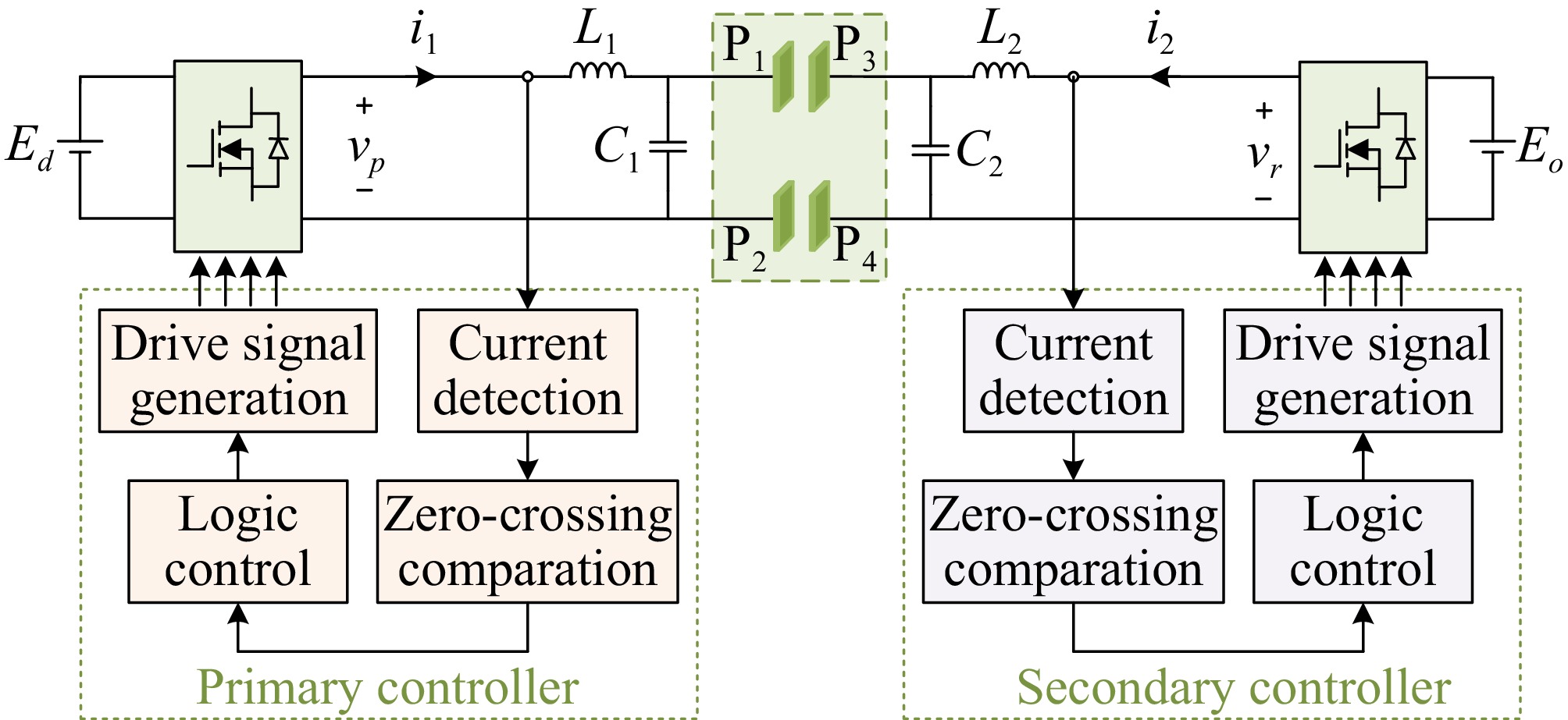
Figure 9.
The proposed frequency tracking control schematic diagram of the bidirectional EC-WPT system.
-
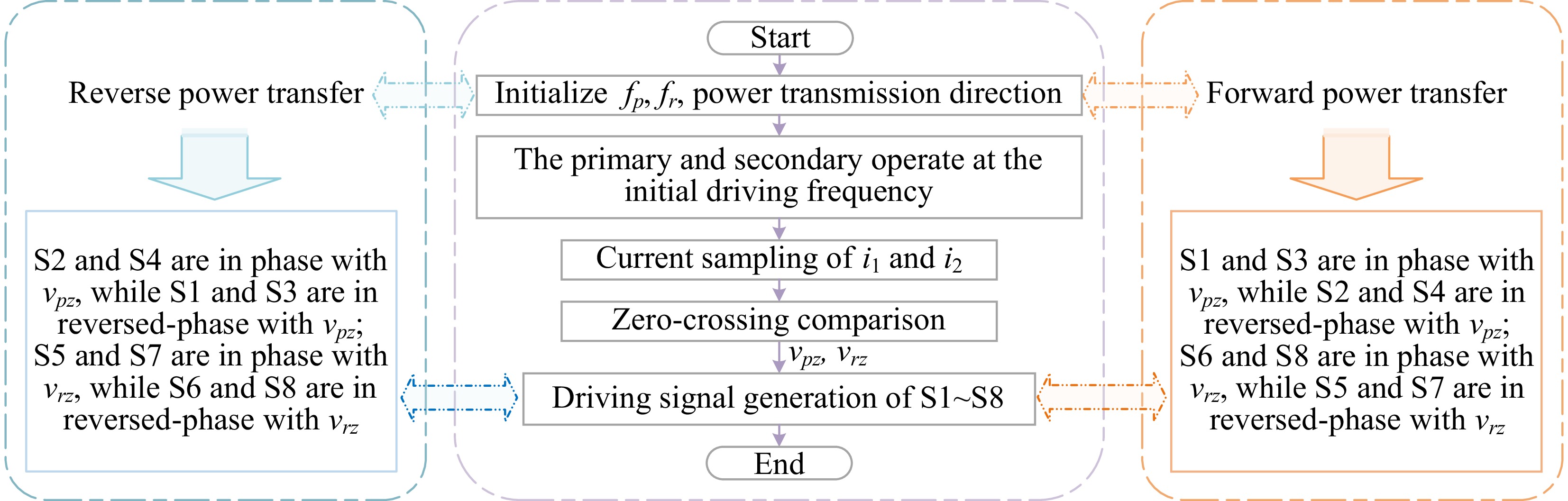
Figure 10.
Procedures of the proposed frequency tracking control schematic.
-
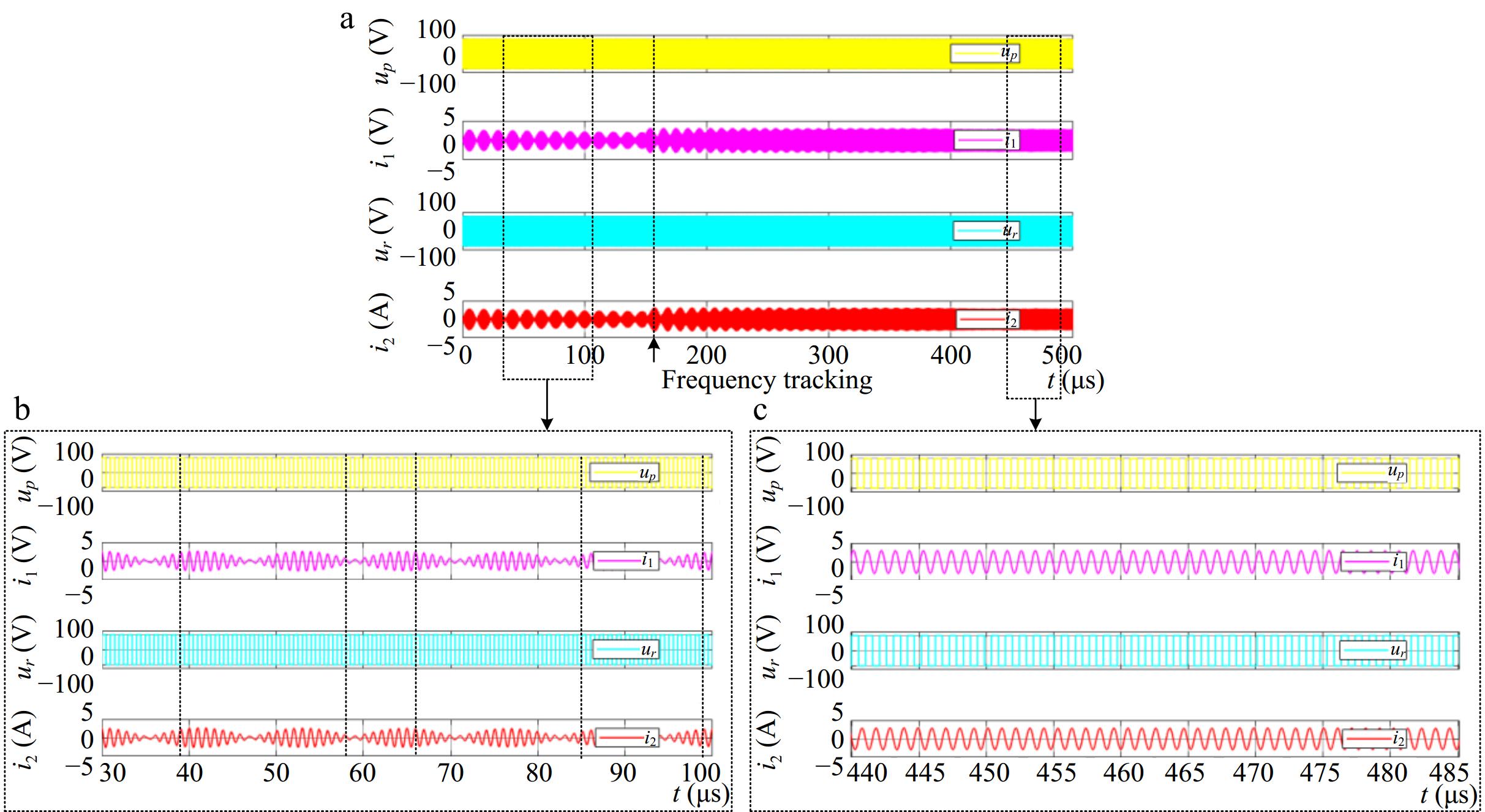
Figure 11.
Resonant voltages and currents generated by the primary and secondary sides of the bidirectional EC-WPT system. (a) Full view of the transient responder. (b) Zoomed-in view of the fixed-frequency driving. (c) Zoomed-in view of the frequency tracking method.
-
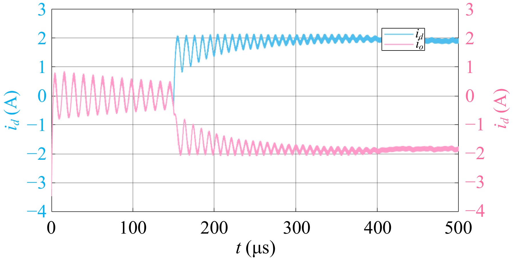
Figure 12.
DC output currents of the primary and secondary sides.
-
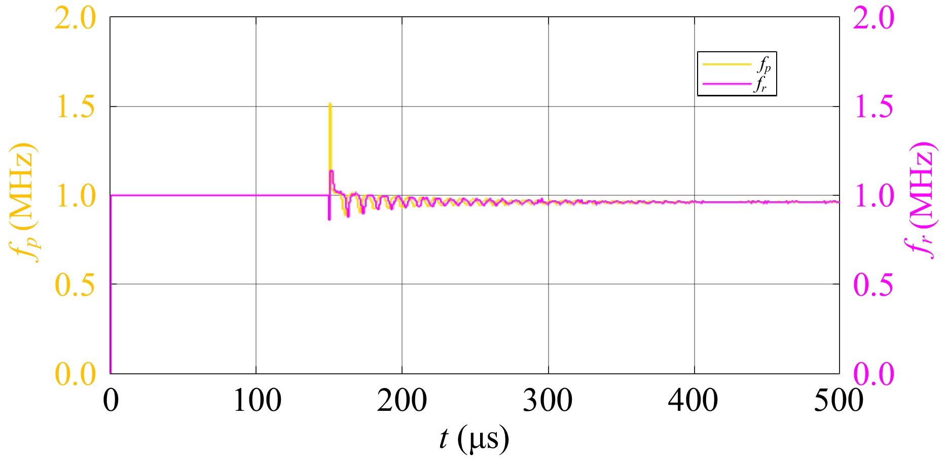
Figure 13.
The operating frequency of the system.
-
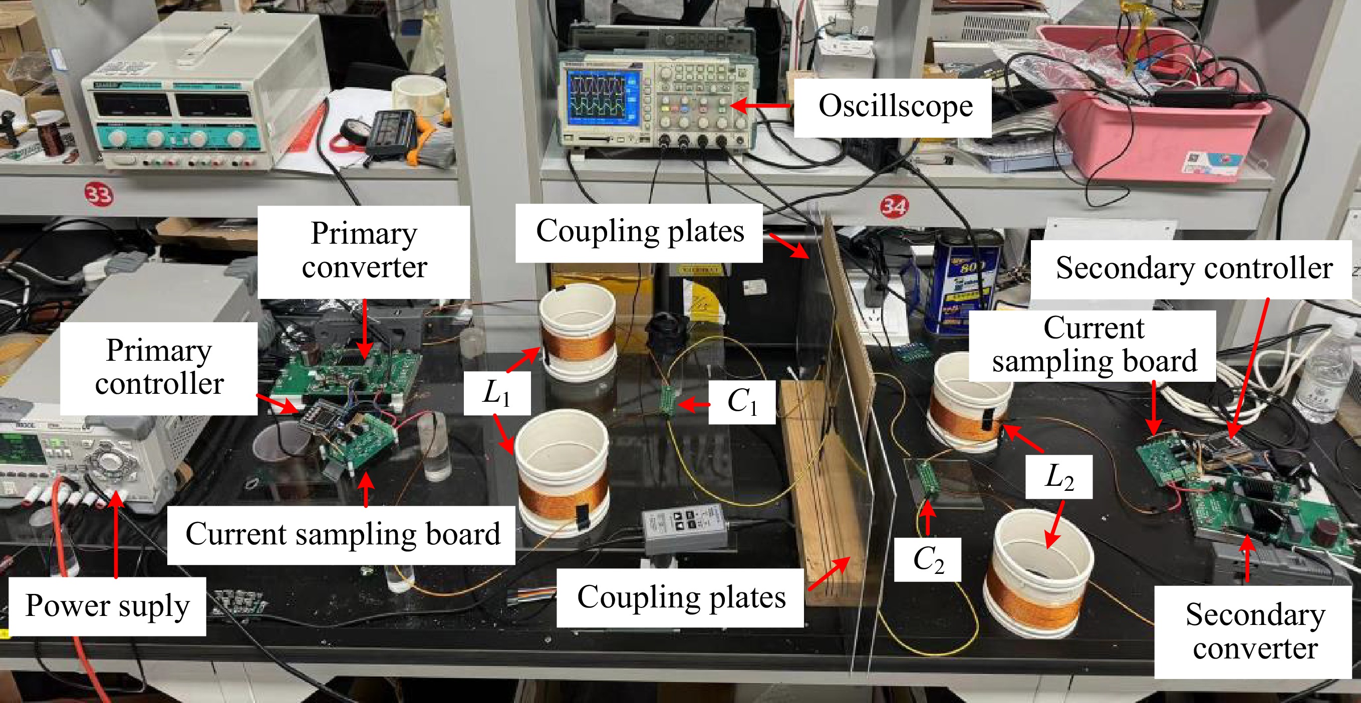
Figure 14.
Experimental prototype of a bilateral LC-compensated bidirectional EC-WPT system.
-
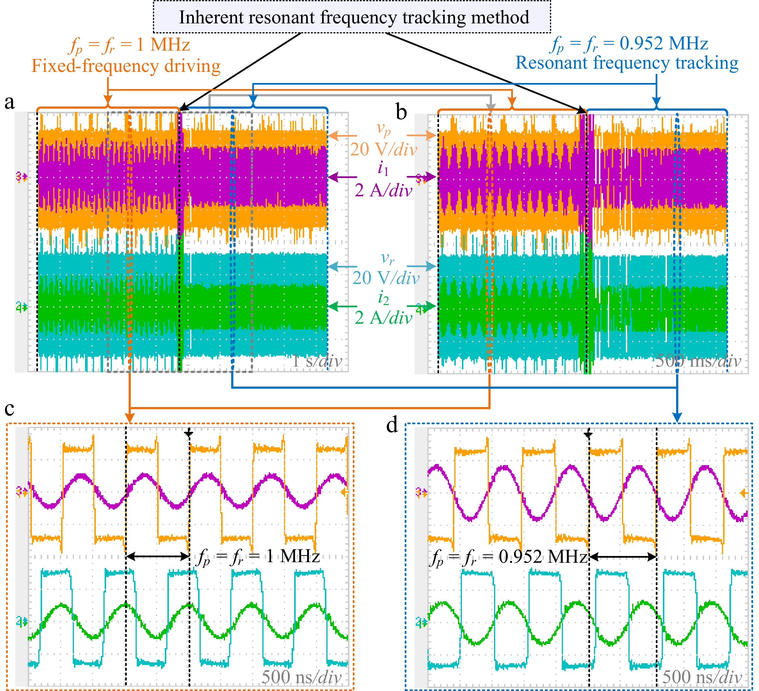
Figure 15.
Resonant voltages and currents generated by the primary and secondary converters. (a) Full view of the transient responder. (b) Zoomed-in view of the transient responder (c) Zoomed-in view of the fixed-frequency driving. (d) Zoomed-in view of thefrequency tracking method.
-
Ref. Method Design complexity Adjustable precision Misalignment tolerability Power disturbance [15] Capacitance matrix platform Medium Low Medium No [9] Dynamic adjustable inductor Medium Low Low No [16] hybrid parallel connected topology High Medium Low No [17] LC-CLC compensation network Medium Low Low Yes [18] Power-phase angle perturbation Medium Medium High Yes This work Autonomously track zero-crossing point of the current low High High No Table 1.
Comparison of critical characteristics of the proposed method and conventional methods.
-
β-δ θ $\varphi $ β < δ (−2π, −π] δ + ( $\varphi $ $\varphi $ β − δ + 2π (−π, 0) δ − ( $\varphi $ $\varphi $ −(β − δ) β > δ (0, π] δ + ( $\varphi $ $\varphi $ β − δ (π, 2π) δ − ( $\varphi $ $\varphi $ − (β − δ) + 2π Table 2.
The relationship of the phase-shift angles.
-
Parameter Value Parameter Value C12 (pF) 91.3 C34 (pF) 90.56 C13 (pF) 1.62 C24 (pF) 1.62 C14 (pF) 1.38 C23 (pF) 1.38 Cx1 (pF) 47.77 Cx2 (pF) 47.77 CM (pF) 44.77 Table 3.
The parameters of coupling capacitances.
-
Parameter Value Ed (V) 100 Eo (V) 100 L1 (μH) 75 L2 (μH) 75 C1 (pF) 284 C2 (pF) 284 Table 4.
Circuit parameters of the system.
Figures
(15)
Tables
(4)