Back Article

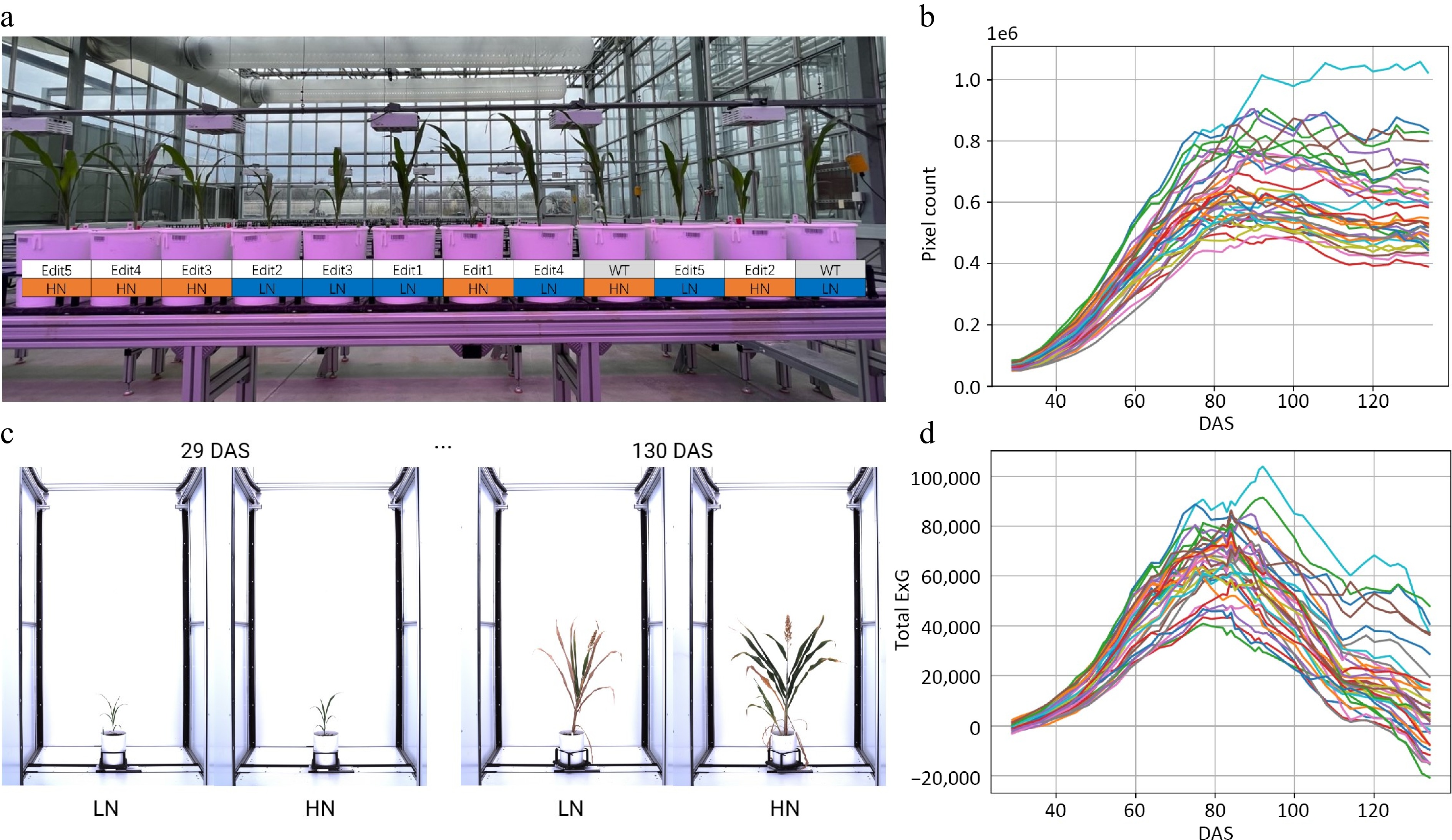
Figure 1. 

Characterizing sorghum CRISPR mutants for N responses using a high-throughput phenotyping procedure. (a) The greenhouse experimental design for CRISPR mutants under high N (15 mM) and low N (3 mM) conditions. (b) Time-series automatic image acquisition from the first day of phenotyping (29 DAS) to the last day of phenotyping (130 DAS). The examples are Tx430 WT. The extracted phenotypes. (c) Pixel count. (d) Total ExG index value for each individual during the phenotyping period.

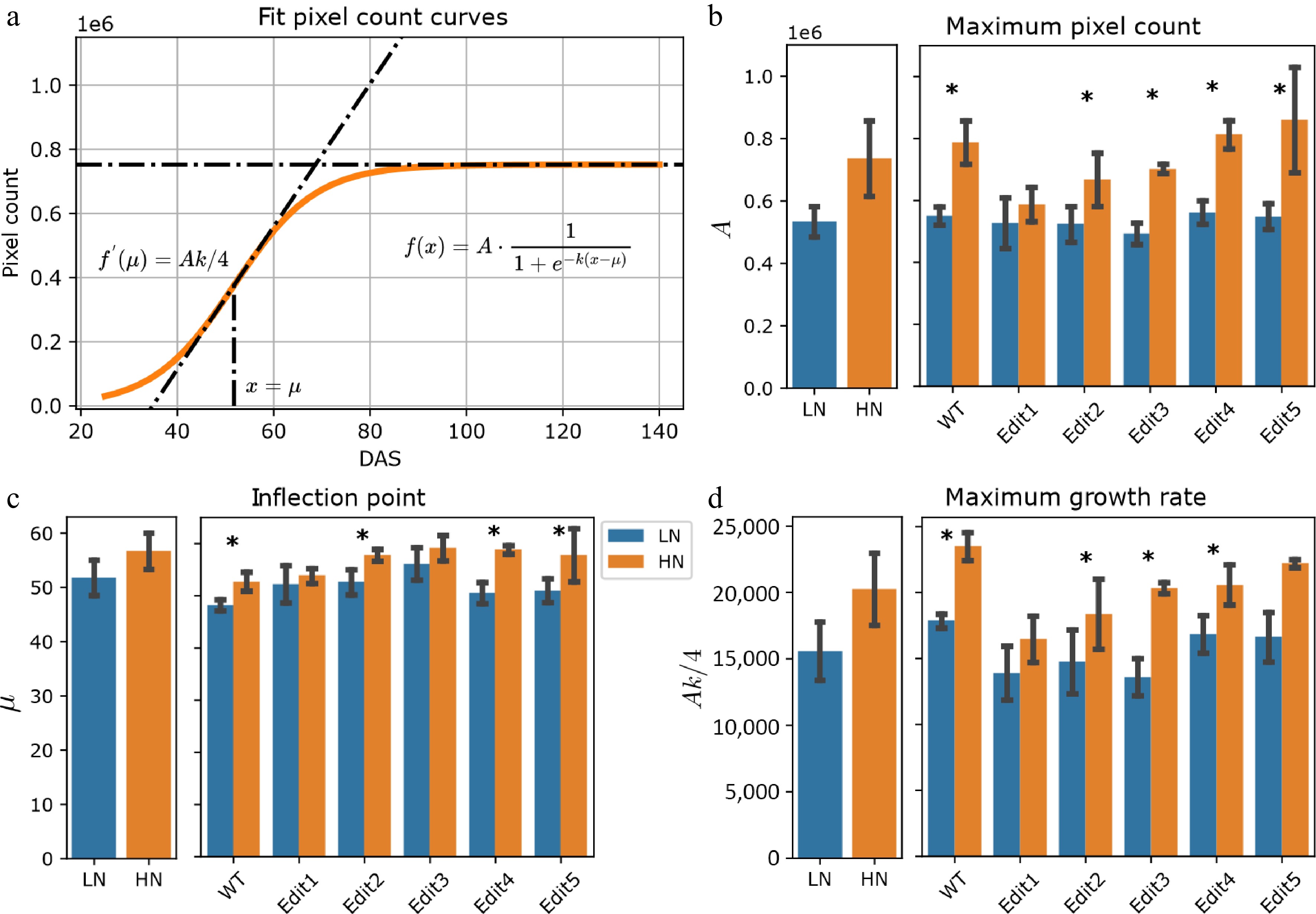
Figure 2. 

Modeling of the pixel count trait. (a) Logistic curves with the parameters estimated from the data. The bold lines represent the curves of WT Tx430 plants, and the dashed color lines represent the gene-edited lines. (b)−(d) The phenotypes estimated or derived from the function. The left panel shows the overall comparisons between treatment and the right panel shows the comparisons for each genotype. The error bars indicate the standard deviation. Stars indicate a significant difference between low N and high N treatment for the pooled data or within a single genotype.

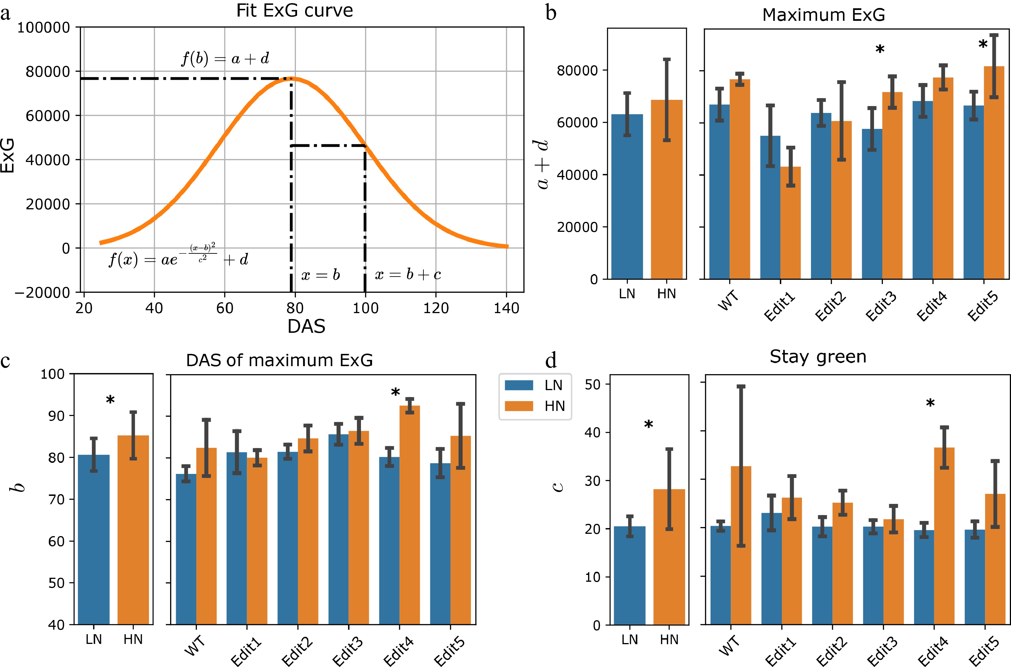
Figure 3. 

Modeling of the ExG index. (a) Fitting the ExG curve as a Gaussian curve and extraction of meaningful phenotypes. (b)−(d) The comparisons of the extracted phenotypes between N treatments. The left panel shows the overall comparisons between treatment and the right panel shows the comparisons for each genotype. The error bars indicate the standard deviation. Stars indicate a significant difference between low N and high N treatment for the pooled data or within a single genotype.