-
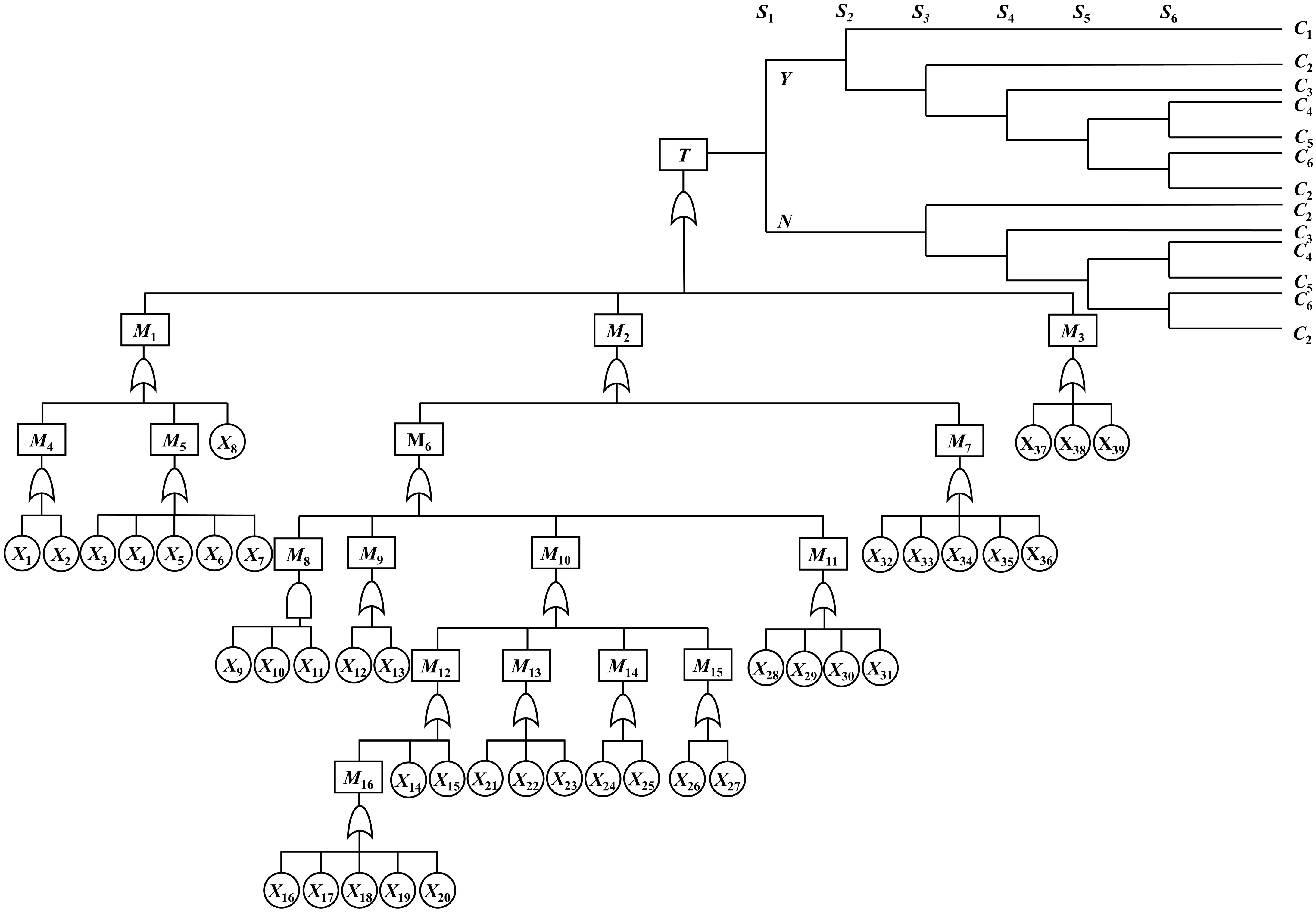
Figure 1.
Syngas pipeline leak BT model.
-
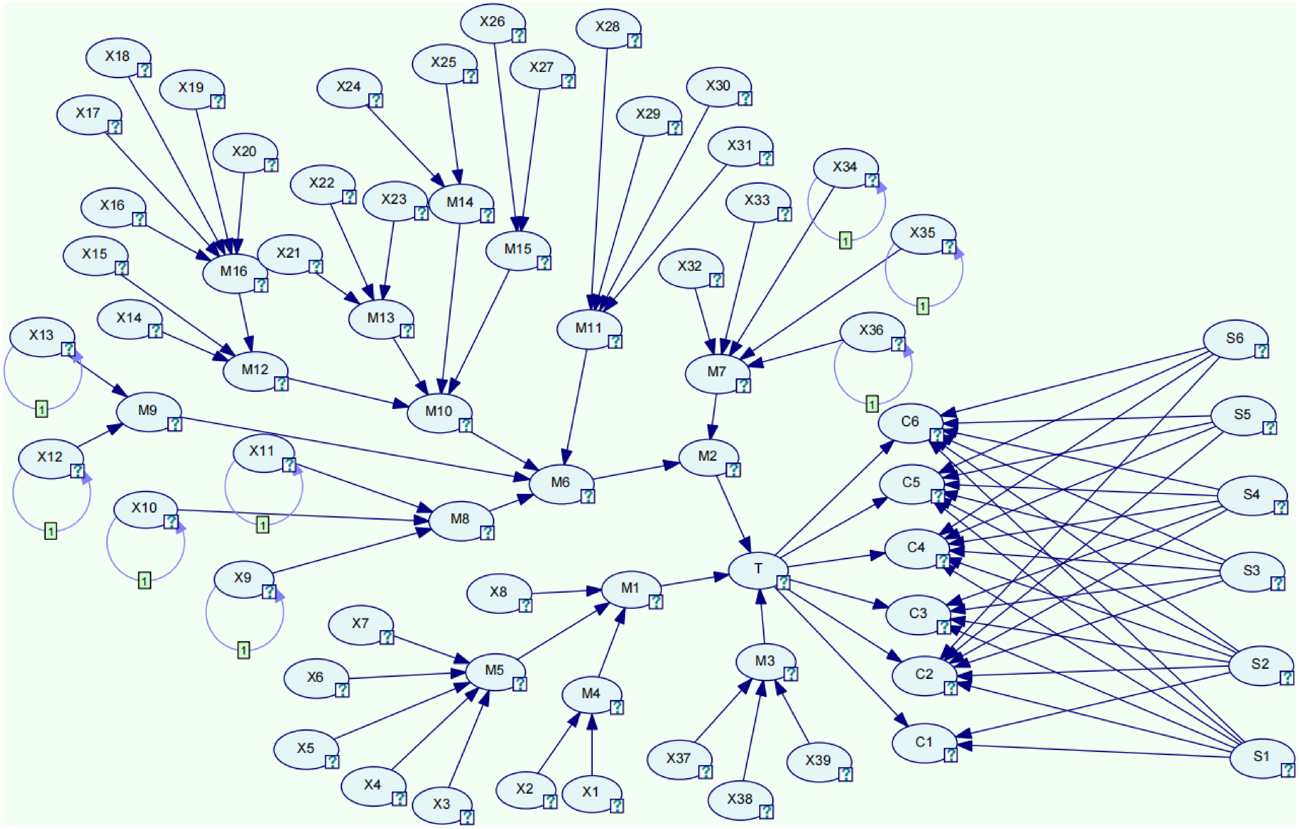
Figure 2.
Bayesian structure chart.
-
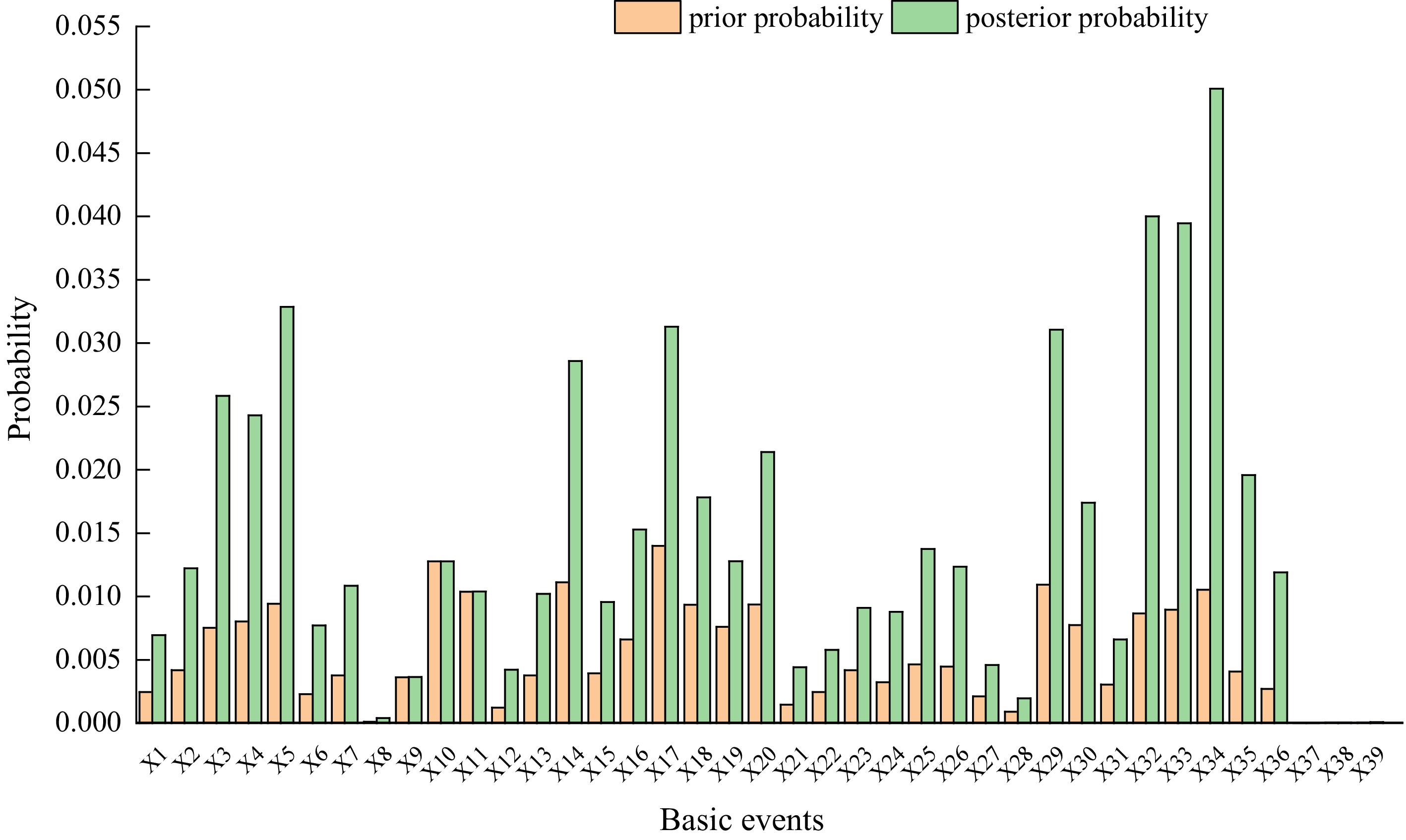
Figure 3.
Comparison of the prior and posterior probabilities of basic events.
-
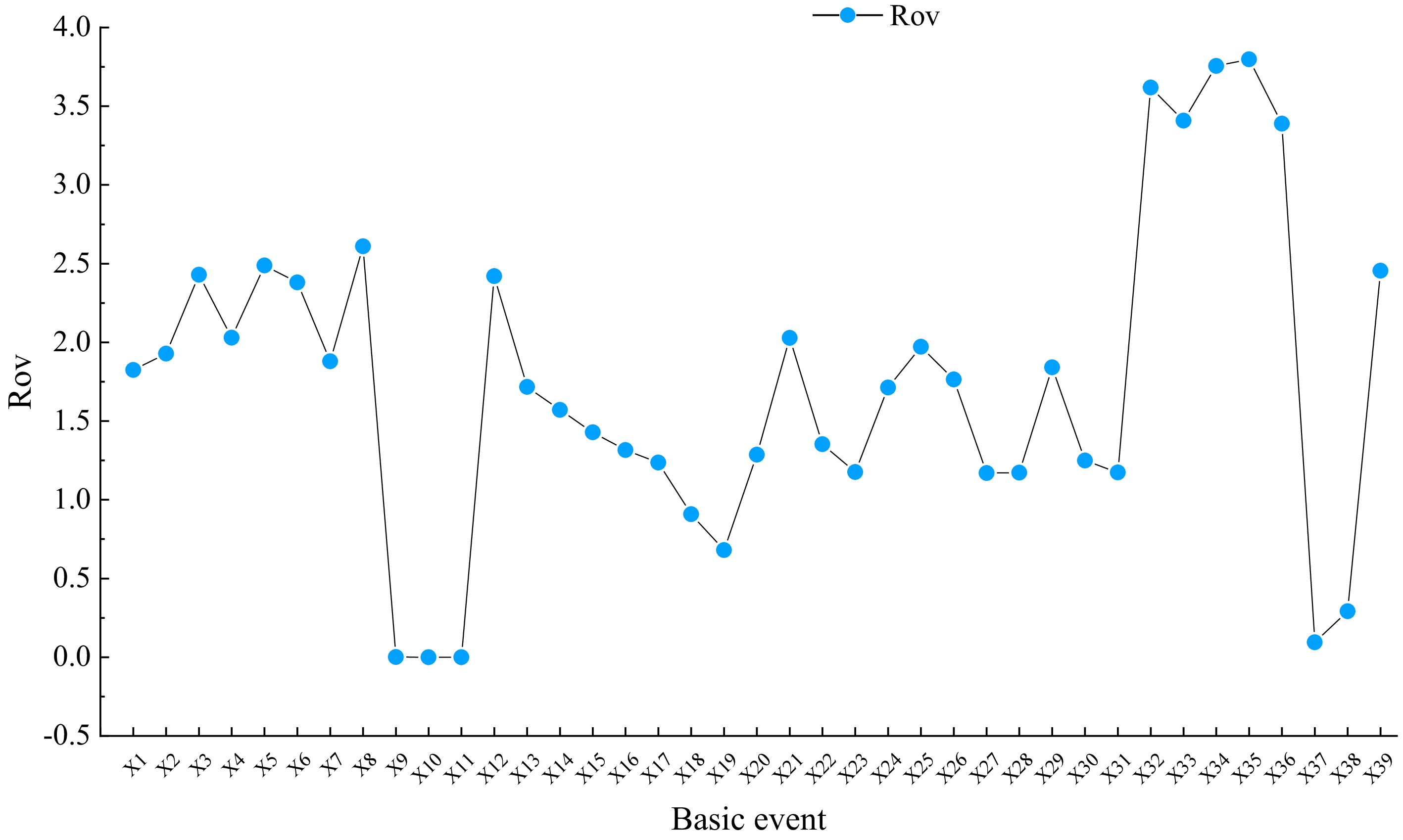
Figure 4.
Basic event RoV value.
-
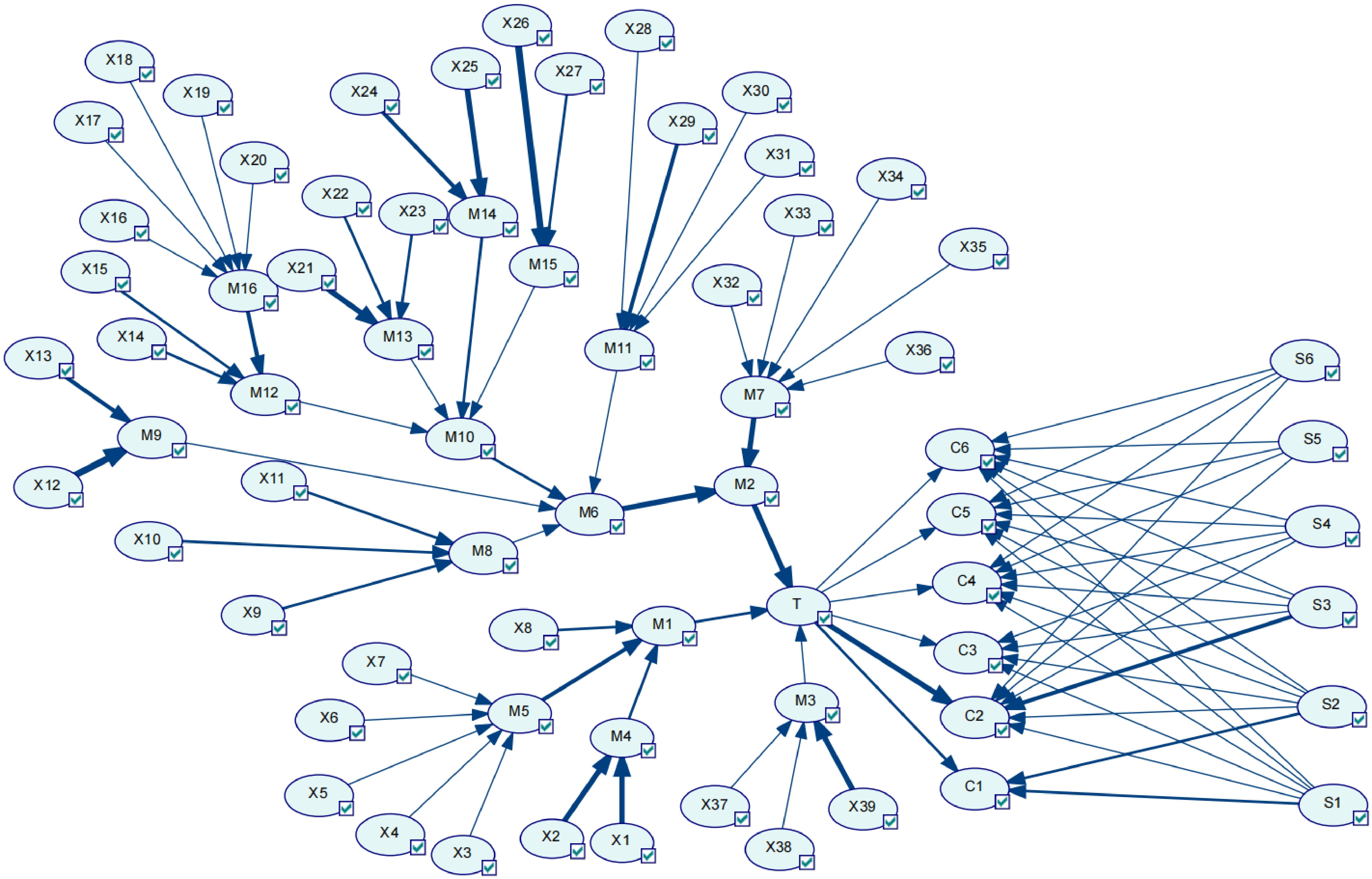
Figure 5.
Causal chain analysis.
-
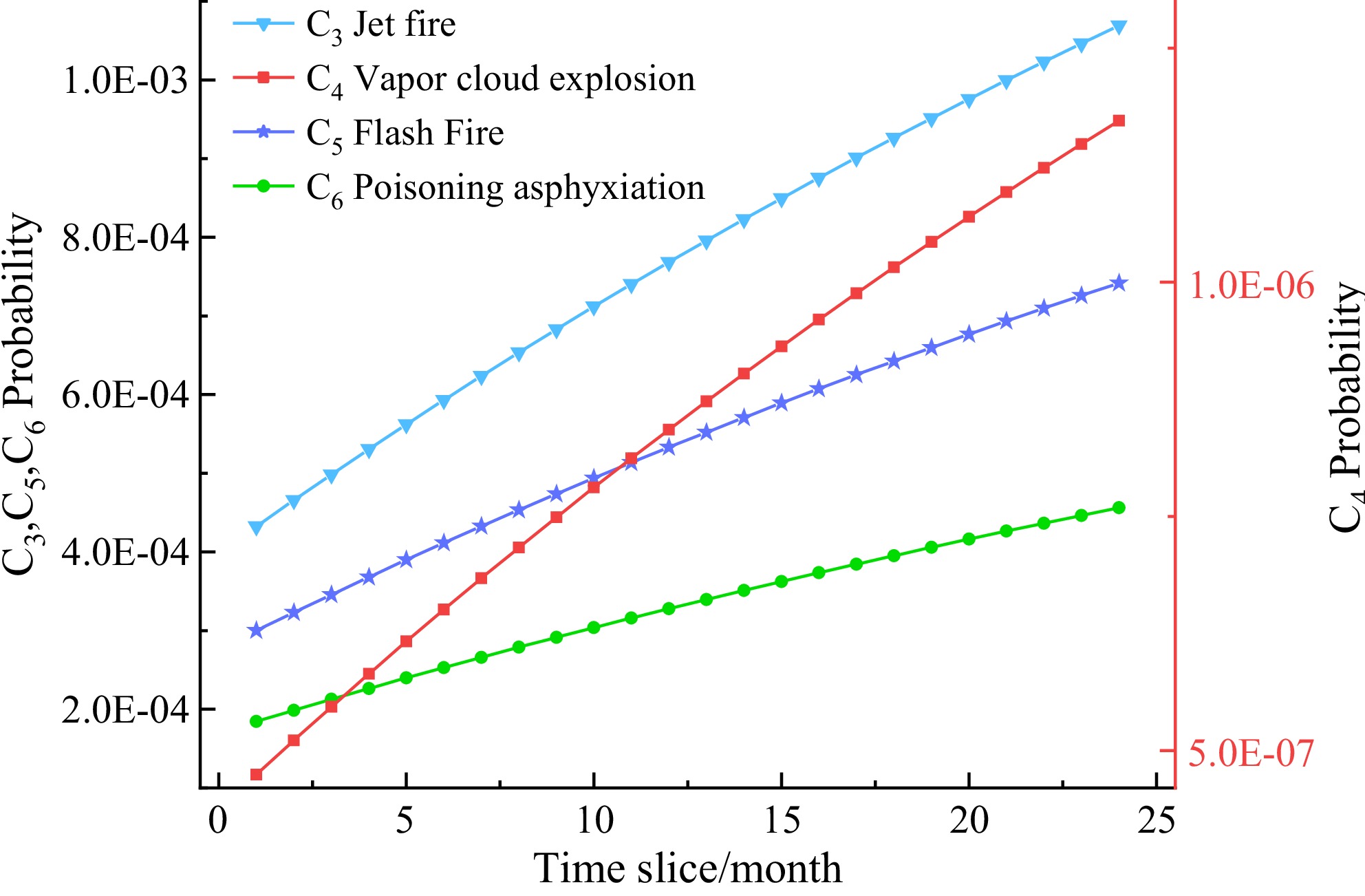
Figure 6.
Changes in probability of consequences of syngas leaks.
-
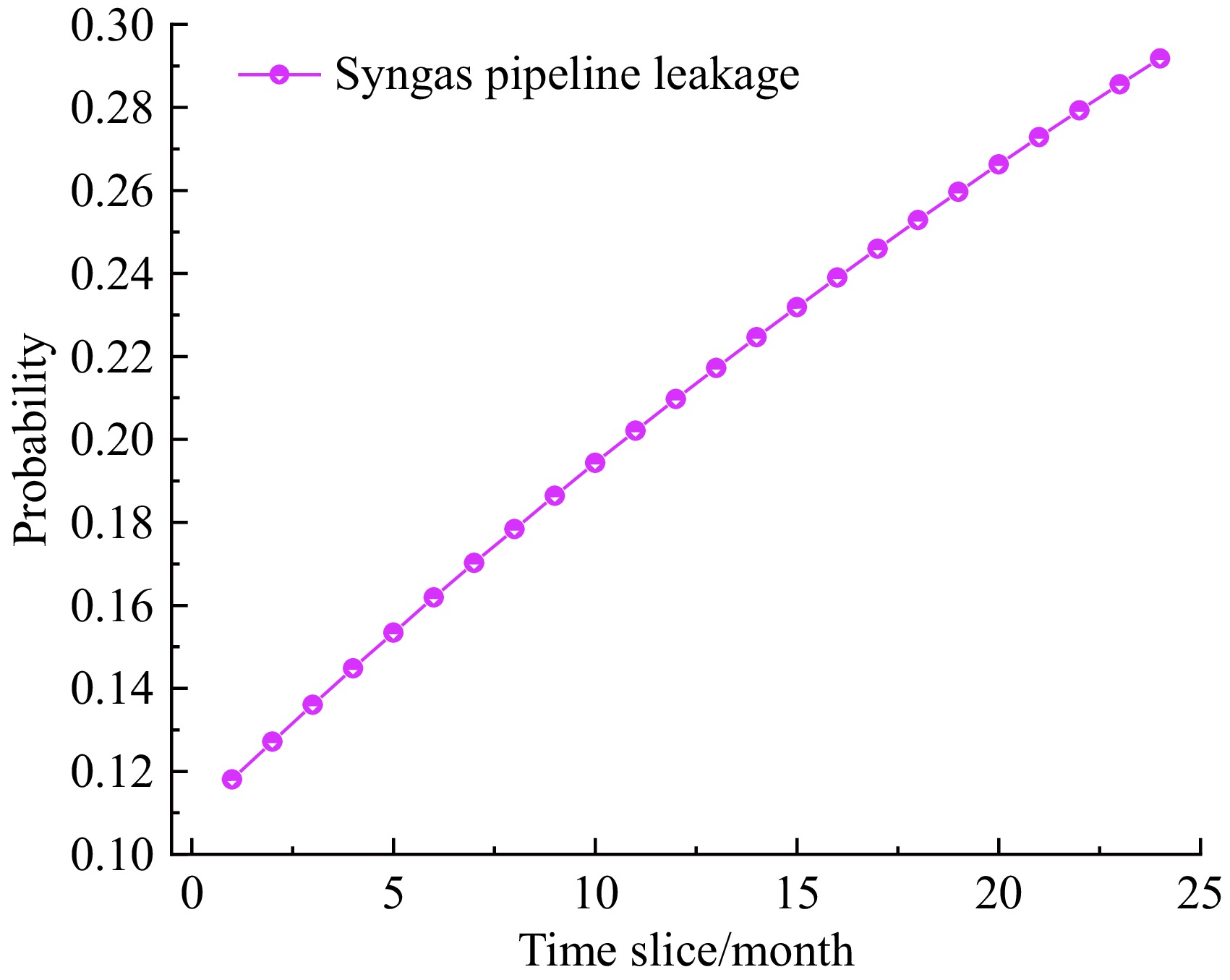
Figure 7.
Change in probability of syngas leakage.
-
Natural language terms and codes Fuzzy intervals (a, b, c, d) VL (0, 0, 0.1, 0.2) L (0.1, 0.2, 0.2, 0.3) ML (0.2, 0.3, 0.4, 0.5) M (0.4, 0.5, 0.5, 0.6) MH (0.5, 0.6, 0.7, 0.8) H (0.7, 0.8, 0.8, 0.9) VH (0.8, 0.9, 1, 1) Table 1.
Transformation of expert opinion into fuzzy numbers.
-
Factor Grade Weight Title Professor/Chief engineer 5 Associate Professor/Senior engineer 4 Lecturer/Engineer 3 Technician 2 Laborer 1 Educational background Doctoral degree 5 Master's degree 4 Bachelor's degree 3 Senior high school 2 Junior high school and below 1 Years of service > 20 years 5 15−20 years 4 10−15 years 3 5−10 years 2 < 5 years 1 Table 2.
Rules for scoring the importance of experts.
-
Code name Descriptive Code name Descriptive T Gasifier syngas pipeline leakage M12 Low liquid level in the cooling chamber M1 Human factors M13 Furnace temperature increase M2 Equipment factors M14 Burn-through of drop tube M3 Environmental factor M15 Clogged pipes M4 Lack of safety awareness M16 Low flow rate of cooling water M5 Error of judgment C1 Security M6 Syngas pipeline leakage C2 Security proliferation M7 Leakage of related accessories C3 Jet fire M8 Pipeline corrosion C4 Vapor cloud explosion M9 Pipe erosion and wear C5 Flash fire M10 Pipe overheating C6 Poisoning asphyxiation M11 Pipe quality defects Table 3.
Top, middle, and consequence events in the BT model.
-
Code name Descriptive Prior probability Posterior probability X1 Insufficient operational experience 2.4594 × 10⁻³ 6.9466 × 10−3 X2 Inadequate pre-service training 4.1776 × 10⁻³ 1.2228 × 10−2 X3 Inadequate inspection 7.5334 × 10⁻³ 2.5832 × 10−2 X4 Quality control is not strict 8.0194 × 10⁻³ 2.4290 × 10−2 X5 Inspection and disassembly is not strict 9.4218 × 10⁻³ 3.2870 × 10−2 X6 Emergency response not in place 2.2802 × 10⁻³ 7.7090 × 10−3 X7 Operational errors 3.7668 × 10⁻³ 1.0847 × 10−2 X8 Third party destruction 1.1149 × 10⁻⁴ 4.0252 × 10−4 X9 Failure of corrosion protection layer 3.6306 × 10⁻³ 3.6320 × 10−3 X10 Corrosive media 1.2773 × 10⁻² 1.2775 × 10−2 X11 Stress corrosion 1.0382 × 10⁻² 1.0383 × 10−2 X12 High coal ash content 1.2346 × 10⁻³ 4.2221 × 10−3 X13 Syngas carries water flushing 3.7584 × 10⁻³ 1.0209 × 10−2 X14 Malfunction of black water regulating valve 1.1120 × 10⁻² 2.8586 × 10−2 X15 Severe water carryover of process gas 3.9371 × 10⁻³ 9.5605 × 10−3 X16 Abnormalities in the cooling pump 6.6038 × 10⁻³ 1.5291 × 10−2 X17 Blackwater filter clogged 1.3997 × 10⁻² 3.1299 × 10−2 X18 Clogging of the cooling ring 9.3452 × 10⁻³ 1.7828 × 10−2 X19 Clogged make-up water pipe 7.6128 × 10⁻³ 1.2786 × 10−2 X20 Abnormality of cooling water regulating valve 9.3608 × 10⁻³ 2.1401 × 10−2 X21 Coal line line breaks 1.4587 × 10⁻³ 4.4175 × 10−3 X22 Oxygen regulator valve failure 2.4594 × 10⁻³ 5.7867 × 10−3 X23 Coal quality change 4.1820 × 10⁻³ 9.0992 × 10−3 X24 Slag hanging on the descending pipe 3.2415 × 10⁻³ 8.7956 × 10−3 X25 Deformation of the cooling ring 4.6277 × 10⁻³ 1.3752 × 10−2 X26 Internal scaling 4.4655 × 10⁻³ 1.2345 × 10−2 X27 Foreign body blockage 2.1168 × 10⁻³ 4.5925 × 10−3 X28 Design defects 9.0316 × 10⁻⁴ 1.9623 × 10−3 X29 Welding defects 1.0935 × 10⁻² 3.1067 × 10−2 X30 Improper material 7.7409 × 10⁻³ 1.74125 × 10−2 X31 Life limitation 3.0448 × 10⁻³ 6.6177 × 10−3 X32 Gasket failure 8.6622 × 10⁻³ 4.0003 × 10−2 X33 Seal failure 8.9526 × 10⁻³ 3.9465 × 10−2 X34 Flange scouring and wear 1.0531 × 10⁻² 5.0083 × 10−2 X35 Valve scouring and wear 4.0810 × 10⁻³ 1.9578 × 10−2 X36 Accessory deterioration 2.7119 × 10⁻³ 1.1904 × 10−2 X37 Typhoon 5.6502 × 10⁻⁶ 6.1817 × 10−6 X38 Earthquake 4.0054 × 10⁻⁵ 5.1756 × 10−5 X39 Other natural disasters 4.0054 × 10⁻⁵ 8.3535 × 10⁻⁵ Table 4.
Basic events in the BT model and the corresponding prior and posterior probabilities.
-
Code name Descriptive Prior probability S1 Monitoring alarms 6.0844 × 10⁻³ S2 Emergency response 2.8469 × 10⁻³ S3 Emergency shutdown 3.4036 × 10⁻³ S4 Immediate ignition 3.6761 × 10⁻³ S5 Delayed ignition 2.5638 × 10⁻³ S6 Restricted space 1.5784 × 10⁻³ Table 5.
Prior probability of safety barrier failure.
-
Natural language (L, M, MH, M, M) $ W({E_i}) $ $ W({E_1}) = \dfrac{{5 + 5 + 3}}{{51}} = 0.255 $ $ \begin{gathered}W(E_1)=0.255;\ W(E_2)=0.235; \\ W(E_3)=0.137;\ W(E_4)=0.137; \\ W(E_5)=0.235 \\ \end{gathered} $ $ S({\tilde A_i},{\tilde A _j}) $ $ \begin{gathered} S({\tilde A _{\text{1}}},{\tilde A _{\text{2}}}) = 1 - \dfrac{1}{4}\sum\nolimits_{i = 1}^4 {\left| {{a_i} - \left. {{b_i}} \right|} \right.} = 1 - \dfrac{1}{4}(0.3 + 0.3 + 0.3 + 0.3) = 0.7 \end{gathered} $ $ \begin{gathered}S(\tilde{A}_{\text{1}},\tilde{A}_{\text{2}})\text{ = 0}\text{.70};\ S(\tilde{A}_{\text{1}},\tilde{A}_{\text{3}})\text{ = 0}\text{.55}; \\ S(\tilde{A}_{\text{1}},\tilde{A}_{\text{4}})\text{ = 0}\text{.70};\ S(\tilde{A}_{\text{1}},\tilde{A}_{\text{5}})\text{ = 0}\text{.70}; \\ ....... \\ \end{gathered} $ $ WA({E_i}) $ $ \begin{aligned} WA({E_{\text{1}}}) =\;& \dfrac{{\displaystyle\sum\nolimits_{{\begin{aligned} j = 1 \\[-5pt] j \ne i \end{aligned}}} ^5 {W({E_j}) \times S({A_i},{A_j})} }}{{\displaystyle\sum\nolimits_{{\begin{aligned} j = 1 \\[-5pt] j \ne i \end{aligned}}} ^5 {W({E_j})} }} = \dfrac{{{\text{0}}{\text{.235}} \times {\text{0}}{\text{.7 + 0}}{\text{.137}} \times {\text{0}}{\text{.55 + 0}}{\text{.137}} \times {\text{0}}{\text{.7 + 0}}{\text{.235}} \times {\text{0}}{\text{.7}}}}{{{\text{0}}{\text{.235 + 0}}{\text{.137 + 0}}{\text{.137 + 0}}{\text{.235}}}} \\ =\;& 0{\text{.6724}} \end{aligned} $ $ \begin{gathered} WA({E_{\text{1}}}) = {\text{0}}{\text{.67238}}; \\ WA({E_{\text{2}}}) = {\text{0}}{\text{.87297}}; \\ WA({E_{\text{3}}}) = {\text{0}}{\text{.76125}}; \\ WA({E_{\text{4}}}) = {\text{0}}{\text{.88741}};\\ WA({E_{\text{5}}}) = {\text{0}}{\text{.87297}} \end{gathered} $ $ RA({E_i}) $ $ \begin{aligned} RA({E_{\text{1}}}) =\;& \dfrac{{WA({E_{\text{1}}})}}{{\displaystyle\sum\nolimits_{i = 1}^5 {WA({E_i})} }} {\text{ = }}\dfrac{{{\text{0}}{\text{.6724}}}}{{{\text{0}}{\text{.67238 + 0}}{\text{.87297 + 0}}{\text{.76125 + 0}}{\text{.88741 + 0}}{\text{.87297}}}} = \dfrac{{{\text{0}}{\text{.67240}}}}{{4.06698}} \\=\;& 0.1653 \end{aligned} $ $ \begin{gathered} RA({E_{\text{1}}}) = {\text{0}}{\text{.1653}}; \\ RA({E_{\text{2}}}) = {\text{0}}{\text{.2146}}; \\ RA({E_{\text{3}}}) = {\text{0}}{\text{.1872}}; \\ RA({E_{\text{4}}}) = {\text{0}}{\text{.2182}}; \\ RA({E_{\text{5}}}) = {\text{0}}{\text{.2146}} \end{gathered} $ $ CC({E_i}) $ $ \begin{array}{c}CC({E}_{1})=\beta \times W({E}_{1})\text{+}({1-}\beta)\times RA({E}_{1}) =0.5\times 0.255+0.5\times 0.1653 =0.2102\end{array} $ $ \begin{gathered} CC({E_{\text{1}}}) = {\text{0}}{\text{.2102}}; CC({E_{\text{2}}}) = {\text{0}}{\text{.2248}}; \\ CC({E_{\text{3}}}) = {\text{0}}{\text{.1621}}; CC({E_{\text{4}}}) = {\text{0}}{\text{.1776}}; \\ CC({E_{\text{5}}}) = {\text{0}}{\text{.2248}} \end{gathered} $ $ \tilde R $ $ \begin{aligned}\tilde{R}=\;&CC({E}_{1})\times {{\tilde A}}_{1}+CC({E}_{2})\times {{\tilde A}}_{2}+\cdot \cdot \cdot +CC({E}_{M})\times {{\tilde A}}_{M} ={0}{.2102}\times (0.1,0.2,0.2,0.3)\\&+\text{0}\text{.2248}\times (0.4,0.5,0.5,0.6) +\text{0}\text{.1621}\times (0.5,0.6,0.7,0.8){+0}{.1776}\times (0.4,0.5,0.5,0.6) \\&+{0}{.2248}\times (0.4,0.5,0.5,0.6) =({0}{.3530}, {0}{.4529}, {0}{.4691}, {0}{.5691})\end{aligned} $ $ \begin{gathered}\text{a}_1\text{ = 0}\text{.3530};\ \text{a}_2\text{ = 0}\text{.4529}; \\ \text{a}_3\text{ = 0}\text{.4691};\ \text{a}_4\text{ = 0}\text{.5691}\end{gathered} $ $ FPS $ $ \begin{aligned} FPS =\;& \dfrac{{\int_{{a_1}}^{{a_{_2}}} {\dfrac{{x - {a_1}}}{{{a_2} - {a_1}}}xdx{\text{ + }}\int_{{a_{\text{2}}}}^{{a_{\text{3}}}} {xdx{\text{ + }}} \int_{{a_{\text{3}}}}^{{a_{_{\text{4}}}}} {\dfrac{{{a_{\text{4}}} - x}}{{{a_4} - {a_3}}}xdx} } }}{{\int_{{a_1}}^{{a_{_2}}} {\frac{{x - {a_1}}}{{{a_2} - {a_1}}}dx{\text{ + }}\int_{{a_{\text{2}}}}^{{a_{\text{3}}}} {dx{\text{ + }}} \int_{{a_{\text{3}}}}^{{a_{_{\text{4}}}}} {\frac{{{a_{\text{4}}} - x}}{{{a_4} - {a_3}}}dx} } }} = \dfrac{1}{3}\dfrac{{{{({a_4} + {a_3})}^2} - {a_4}{a_3} - {{({a_1} + {a_2})}^2} + {a_1}{a_2}}}{{({a_4} + {a_3} - {a_1} - {a_2})}} \\ =\;& \dfrac{1}{3}\frac{{{{(0.5691 + 0.4691)}^2} - 0.5691 \times 0.4691}}{{(0.5691 + 0.4691 - 0.3530 - 0.4529)}} + \dfrac{1}{3}\dfrac{{ - {{(0.3530 + 0.4529)}^2} + 0.3530 \times 0.4529}}{{(0.5691 + 0.4691 - 0.3530 - 0.4529)}} \\=\;& 0.4610 \end{aligned} $ $ FPS = 0.4610 $ $ FFP $ $ \begin{aligned}& K = {\left(\dfrac{{1 - FPS}}{{FPS}}\right)^{1/3}} \times 2.301 = {\left(\frac{{1 - 0.461}}{{0.461}}\right)^{1/3}} \times 2.301 = 2.424{\text{0}} \\ &FFP = \frac{1}{{{{10}^k}}} = \frac{1}{{{{10}^{2.4241}}}} = 0.0037668 \end{aligned} $ $ \begin{gathered} K = 2.424{\text{0}}; \\ FFP = 0.0037668 \\ \end{gathered} $ Table 6.
X7 detailed calculation process.
-
$ P\left( {{X_i}} \right) $ $ \begin{gathered} P\left( {{X_1}} \right) = \dfrac{{P(Y|{X_L}) - P(Y|\bar X)}}{{1 - P(Y|\bar X)}} = \dfrac{{0.875 - 0.238}}{{1 - 0.238}} = 0.836 \end{gathered} $ P(X1) = 0.836; P(X2) = 0.558; P(X3) = 0.486 $ P\left( {{X_i}} \right) $ $ P\left( {{M_{13}}} \right) $ $ \begin{gathered} P({M_{13}} = 1) = 1 - (1 - {P_L}){\prod\nolimits _{i:{X_i} \in {X_p}}}(1 - {P_i}) {\text{ = }}1 - (1 - {\text{0}}{\text{.01}}) \times (1 - {\text{0}}{\text{.836}}) \times (1 - {\text{0}}{\text{.558}}) \times (1 - {\text{0}}{\text{.486}}) = 0.9631 \end{gathered} $ Table 7.
Detailed calculation process.
-
Event X21 X22 X23 P (M13 = 1) P (M13 = 0) Probability 1 1 1 0.9631 0.0369 1 1 0 0.9282 0.0718 1 0 1 0.9164 0.0836 1 0 0 0.8376 0.1624 0 1 1 0.7749 0.2251 0 1 0 0.5625 0.4375 0 0 1 0.4907 0.5093 0 0 0 0.0100 0.9900 Table 8.
M13 conditional probability table.
-
Y N Y 1 0.0066 N 0 0.9934 Table 9.
M13 transfer probability table.
Figures
(7)
Tables
(9)