-
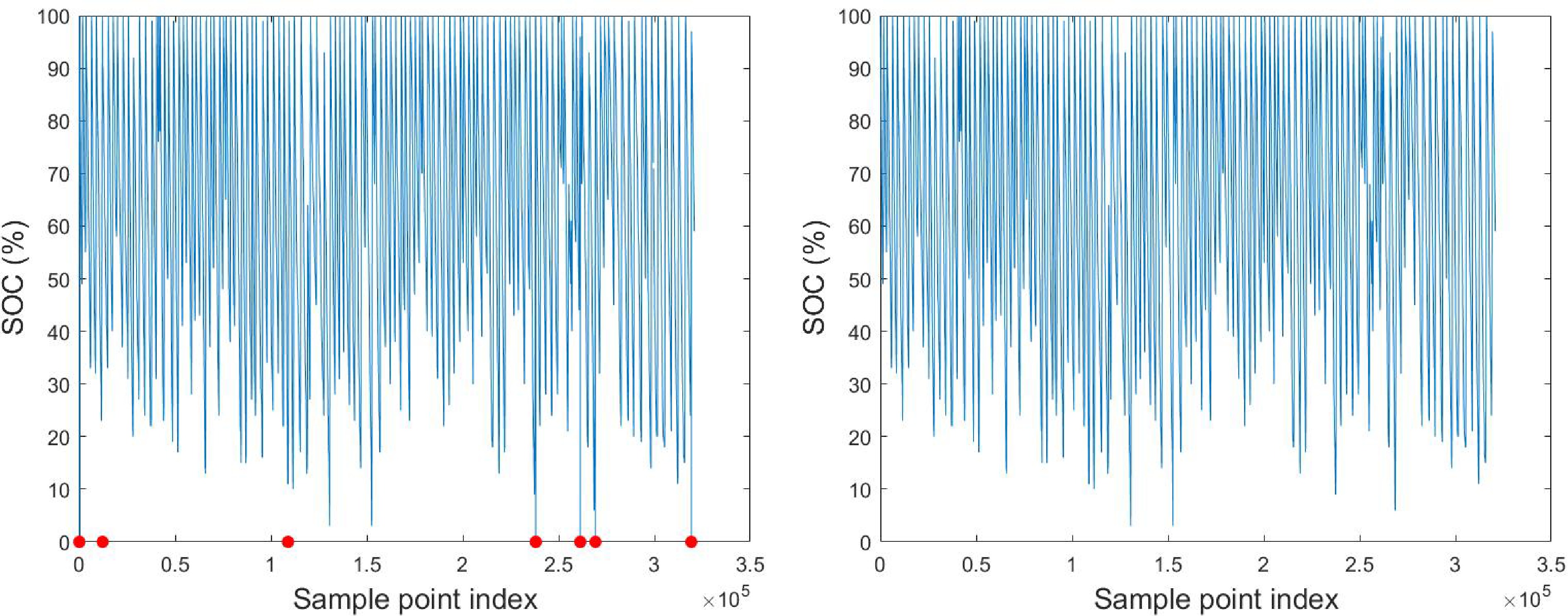
Figure 1.
SOC trends before and after outliers are removed.
-
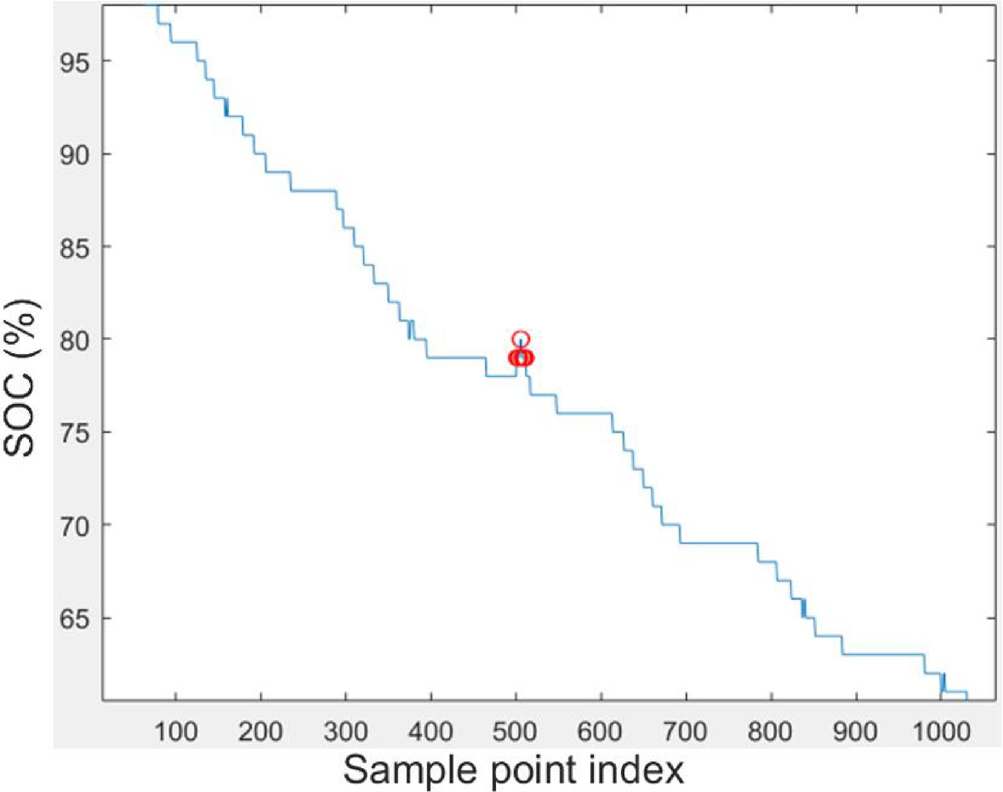
Figure 2.
An example of SOC trend under abnormal conditions.
-
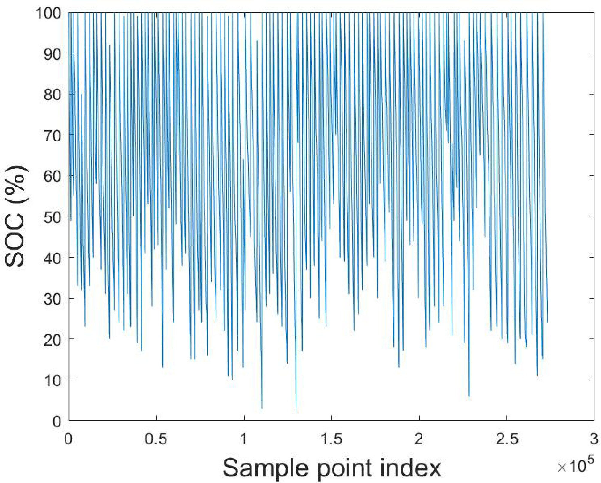
Figure 3.
SOC decreasing trend of processed data.
-
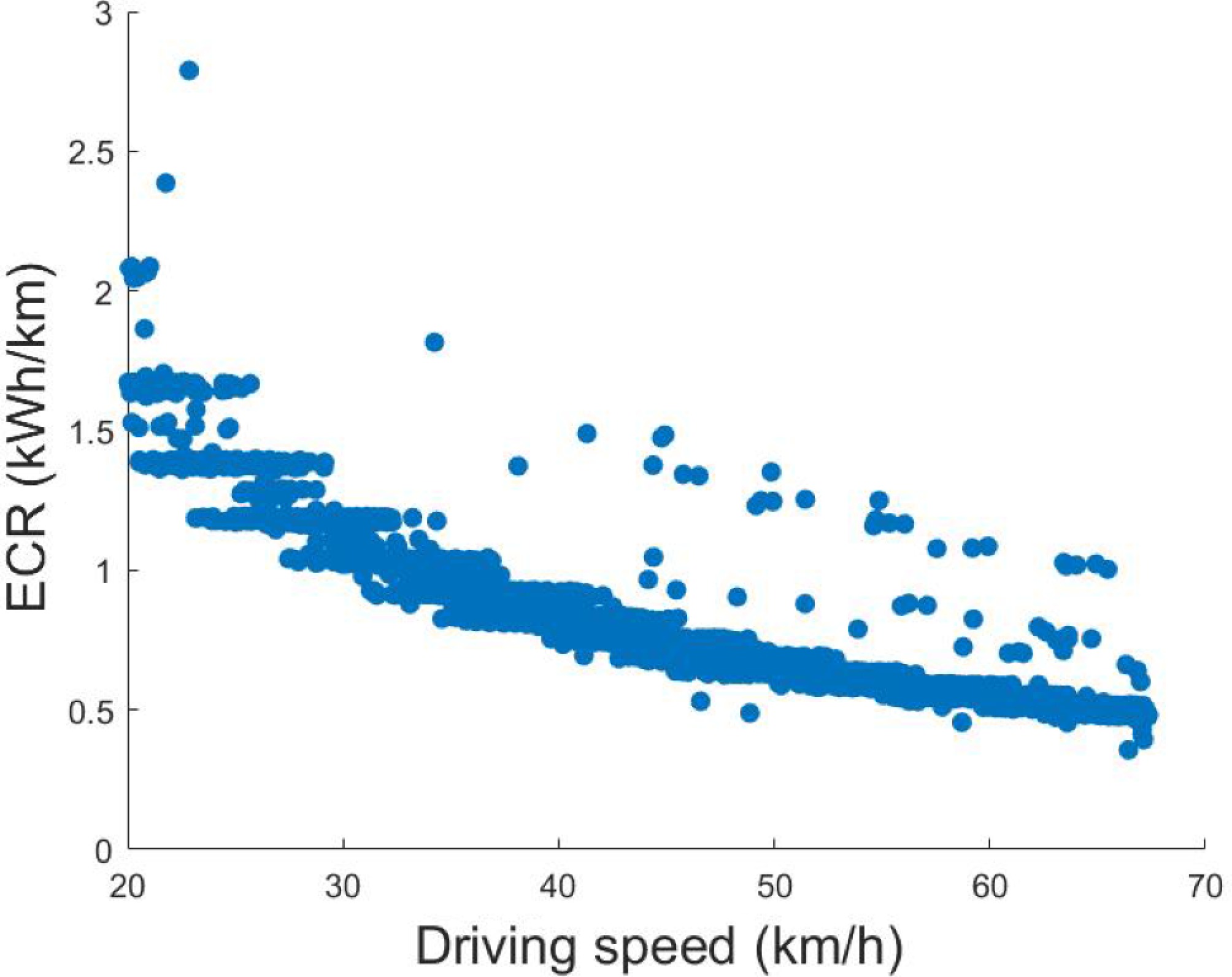
Figure 4.
Scatter plot of the ECR and driving speed.
-
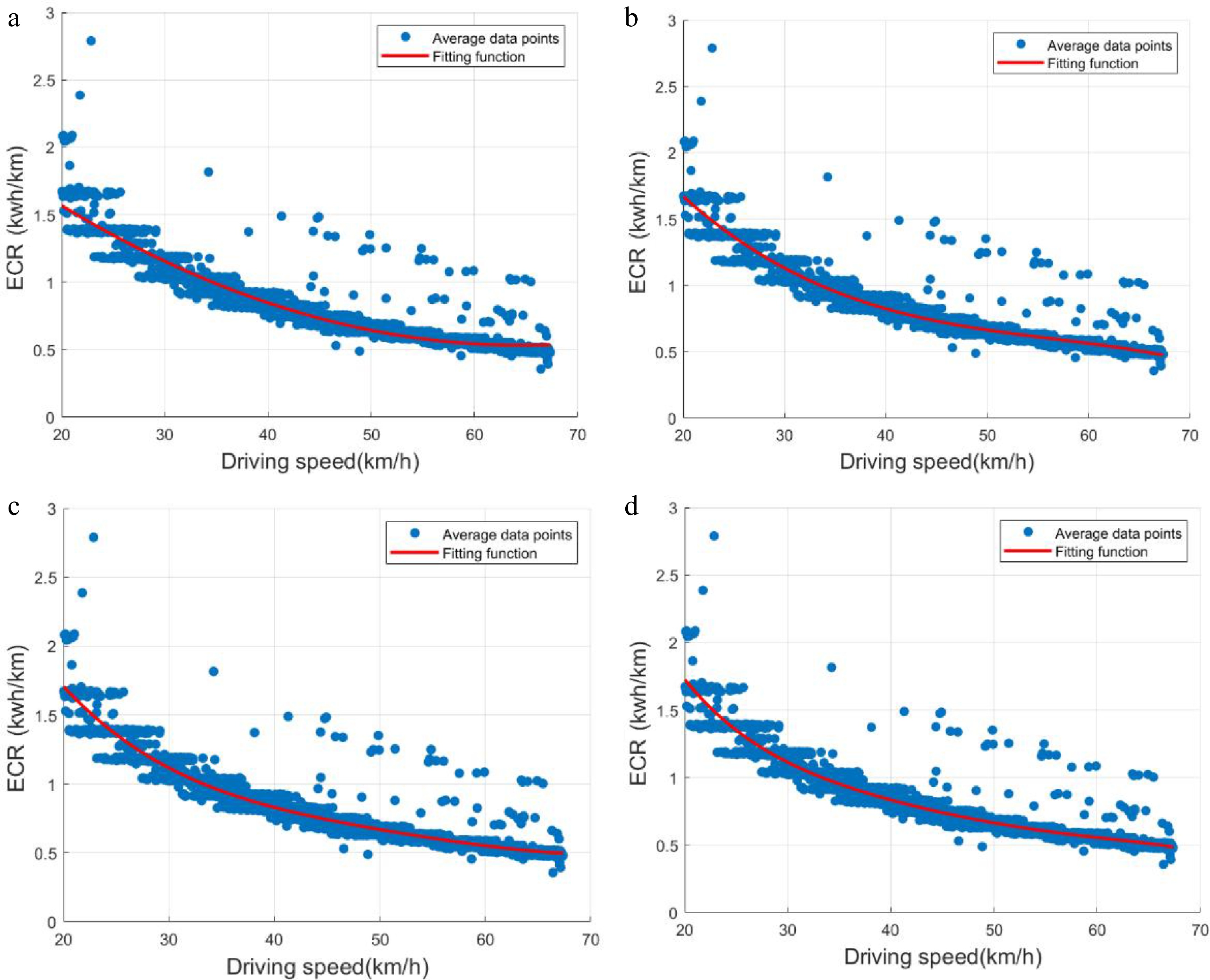
Figure 5.
Fitted curves of the model frameworks. (a) Quadratic function fitting, (b) Cubic function fitting, (c) Quartic function fitting, (d) Quintic function fitting.
-
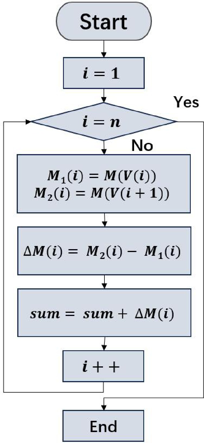
Figure 6.
Flow chart for model verification.
-
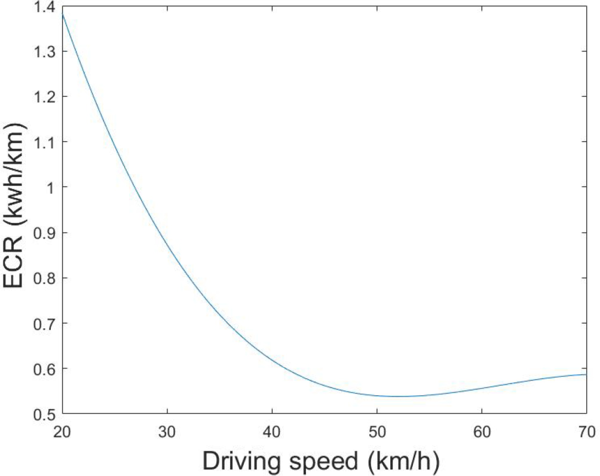
Figure 7.
Change trends of ECR with driving speed.
-
Current (A) Voltage (V) Driving speed (km/h) SOC (%) Mileage (m) 0 563 0 99 19560600 0 563 0 99 19560600 0 563 0 99 19560600 0 563 0 99 19560600 Table 1.
An example of duplicate data.
-
Current (A) Voltage (V) Driving speed (km/h) SOC Mileage (m) NAN NAN NAN NAN NAN 0 562.60 0 99 19560500 5.20 560.90 1.20 99 19560500 NAN NAN NAN NAN NAN Table 2.
An example of missing data.
-
Model framework Quintic coefficient Quartic coefficient Cubic coefficient Quadratic coefficient Linear coefficient Constant term Quadratic 0.0005 −0.0672 2.7038 Cubic −0.000013 0.0025 −0.1505 3.5024 Quartic 0.0000004 −0.00009 0.0071 −0.2765 5.0188 Quintic 0 0.000004 −0.0004 0.0202 −0.5375 7.0127 Table 3.
Parameter values of each model framework.
-
Model framework RMSE R2 $ \overline {RMSE} $ Quadratic function 0.0818 0.9144 0.0856 Cubic function 0.0767 0.9247 0.0823 Quartic function 0.0762 0.9258 0.0629 Quintic function 0.0760 0.9261 0.0831 Table 4.
Metric values for the evaluation of the model frameworks.
Figures
(7)
Tables
(4)