A slower-than-needed scale-up of renewable energy might reduce the incentive for mitigation

Rong Wang; Rong Wang

doi:10.48130/een-0025-0012

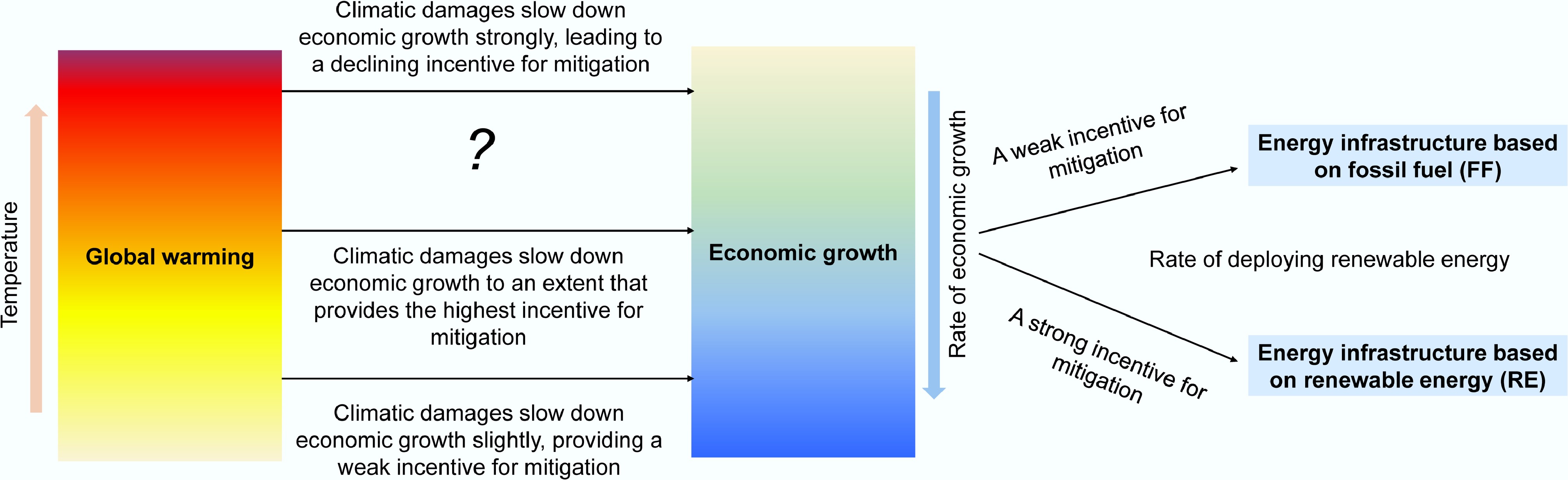
Figure 1.

Schematic illustration of the hypothesis tested in this study. The study examines whether delaying the initiation of strong incentives for mitigation and to phase out fossil fuels could produce a self-reinforcing disincentive, thereby undermining global mitigation efforts.

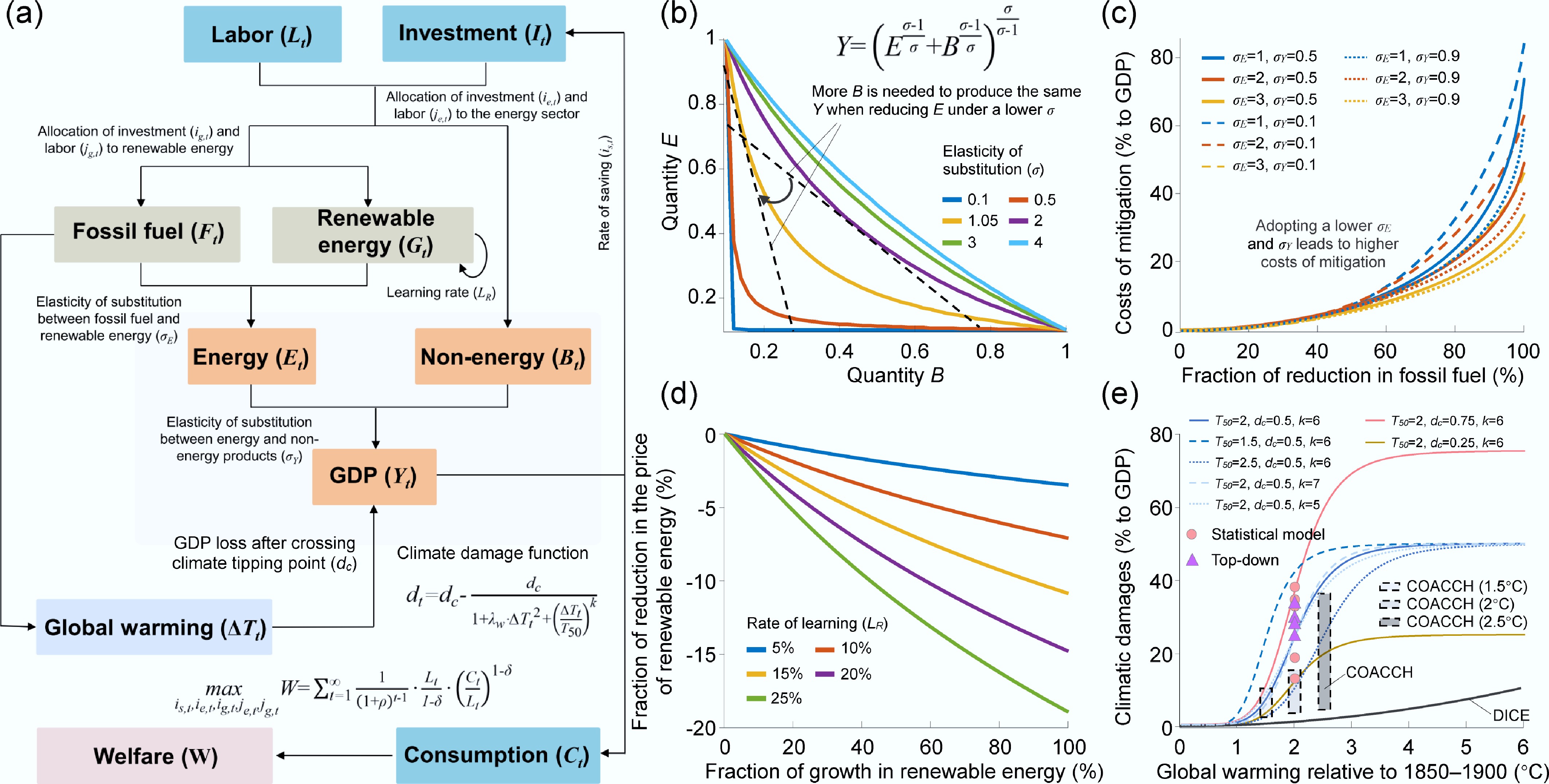
Figure 2.

Economics of climate mitigation. (a) Structure of the integrated assessment model used in this study. (b) Trade-offs between two quantities (E and B) when producing the same output (Y) in the CES function. The variable σ denotes the elasticity of substitution between E and B. The dashed line denotes the marginal increase in E that is needed to offset the effect of reducing B when producing the same output. (c) Dependence of the costs of mitigation as a percentage of GDP on the elasticity of substitution between energy and nonenergy inputs (σ_Y) and the elasticity of substitution between fossil fuel and renewable energy (σ_E). (d) The fraction of decrease in the price of renewable energy resulting from technological advances, based on the learning rate (L_R). (e) Dependence of climatic damage as a percentage of GDP on global warming for different values of the coefficients T₅₀, d_c, and k within the damage function^[23]. For comparison, the black line denotes the damage curve in the Dynamic Integrated Model of Climate and the Economy (DICE) model^[46], the box denotes a bottom-up estimate as a part of CO-designing the Assessment of Climate Cange (COACCH) Project 27, the circle denotes a top-down estimate^[28,29], and the triangle denotes an estimate from a statistical model^[30].

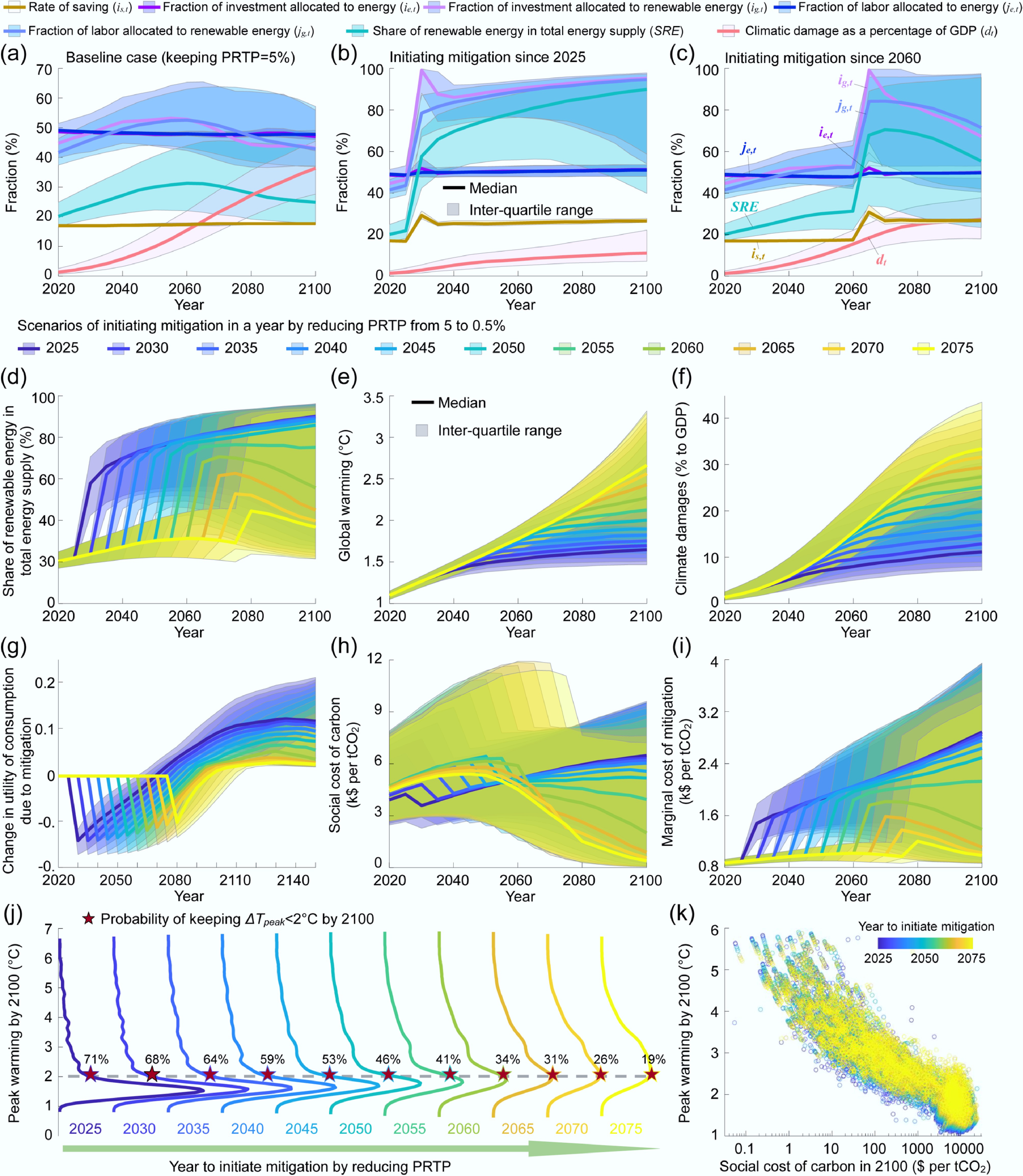
Figure 3.

Economic and climatic impacts of initiating mitigation in a specific year. (a)−(c) Comparison of the temporal trends in the optimal rate of saving, the fraction of labor and investment allocated to produce energy and renewable energy, the share of renewable energy within total energy, and climatic damages as a percentage of GDP between the baseline scenario keeping the pure rate of time preference (PRTP) at 5% (a) and the scenario of mitigation by introducing an impulse reduction in the PRTP from 5% to 0.5% after 2025 (b) or 2060 (c). (d)–(i) Temporal trends in (d) the share of renewable energy, (e) global warming, (f) climatic damage, (g) change in the utility of consumption relative to the baseline scenario, (h) the SCC, and (i) the marginal costs of mitigation in 11 scenarios initiating mitigation in a specific year between 2025 and 2075. (j) Comparison of the probability distribution of peak warming by 2100 in 10,000 Monte Carlo simulations when mitigation is initiated in a specific year between 2025 and 2075. The probability of keeping global warming below 2 °C by 2100 is indicated by the pentagram. (k) Scatter plots of the projected global peak warming by 2100 against the SCC in 2100 in the Monte Carlo simulations. The SCC is calculated as the discounted total damages in the future caused by an increase in tCO₂ emissions at present under a PRTP of 0.5%^[42].

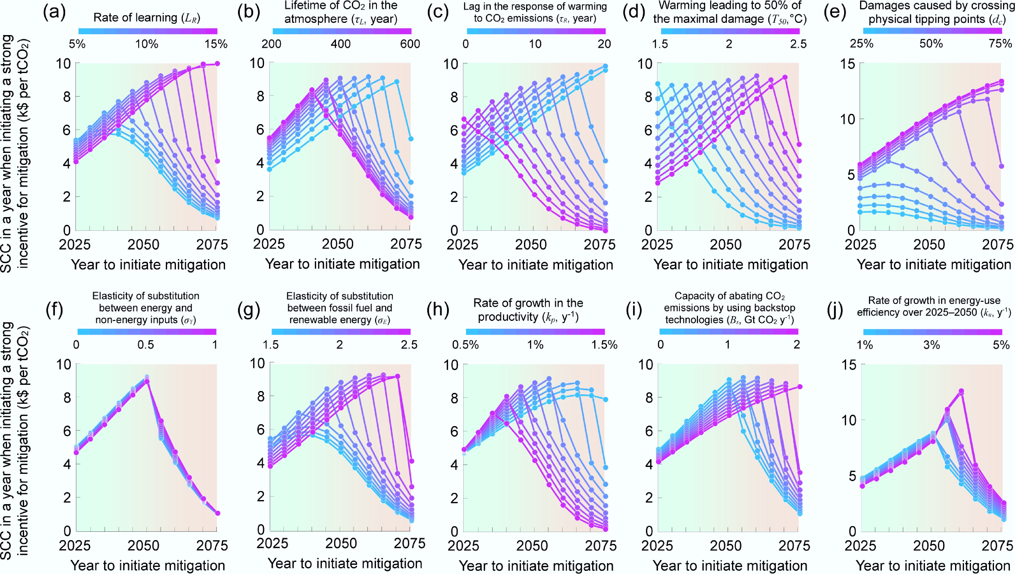
Figure 4.

Sensitivities of the social cost of carbon (SCC) to key parameters in the model. The SCC is calculated for the year when initiating a strong incentive for mitigation in a set of sensitivity experiments which varied (a) the rate of learning (L_R), (b) the atmospheric lifetime of CO₂ (τ_L), (c) lag time of the response of global warming to CO₂ emissions (τ_R), (d) the threshold of global warming for crossing catastrophic tipping points in the climate system (T₅₀), (e) the maximal climatic damage caused by crossing catastrophic tipping points as a percentage of GDP (d_c), (f) the elasticity of substitution between energy and nonenergy inputs (σ_Y), (g) the elasticity of substitution between fossil fuels and renewable energy (σ_E), (h) the rate of growth in the productivity (k_p), (i) capacity of backstop technologies abating emissions at a cost of USD${\$} $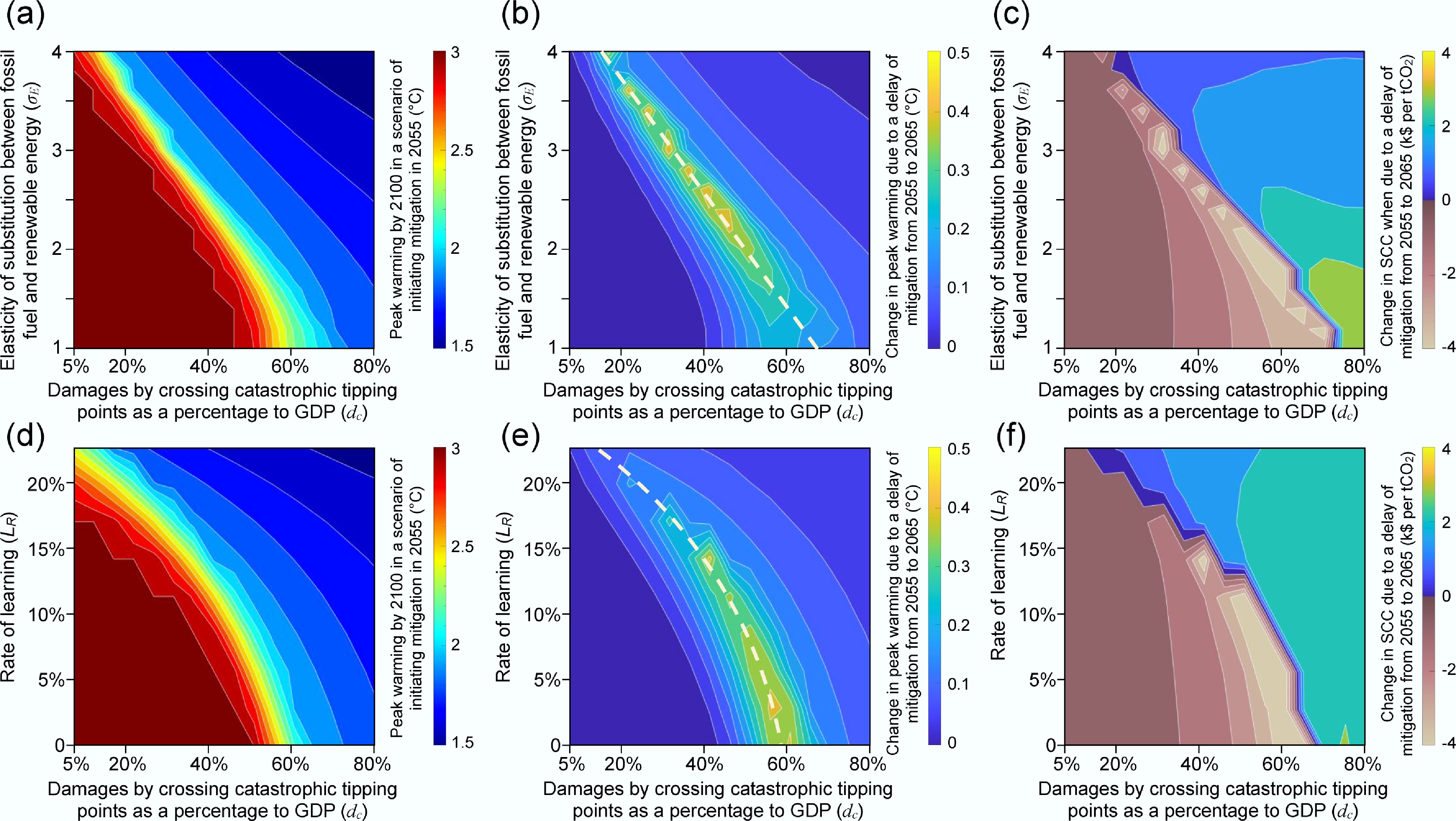100 per tCO₂, and (j) the abrupt increase in energy-use efficiency over 2025−2050 (k_u). The impact of varying each parameter is estimated separately while keeping the other parameters unchanged (L_R= 10%, τ_L= 400 years, τ_R= 10 years, T₅₀= 2 °C, d_c= 50%, σ_Y= 0.5, σ_E= 2, k_p= 1% y⁻¹, B_S= 0, and k_u= 1% y⁻¹). The SCC is estimated under a PRTP of 0.5%⁴² in the optimal path under welfare maximization.

Figure 5.

Responses in the projected peak warming by 2100 and the SCC to a delay in the year of initiating mitigation. (a) Prediction of peak warming by 2100 in scenarios initiating mitigation in 2055 when varying the elasticity of substitution between fossil fuels and renewable energy (σ_E) and the climatic damage caused by catastrophic tipping points (d_c) simultaneously. (b), (c) Responses in (b) the projected peak warming by 2100 and (c) SCC estimated for the year of initiating mitigation to a delay in the year of initiating mitigation from 2055 to 2065 when varying σ_Eand d_c simultaneously. (d) Prediction of peak warming by 2100 in the scenario of initiating mitigation in 2055 when varying the rate of learning (L_R) and d_c simultaneously. (e), (f) Responses in (e) the projected peak warming by 2100 and (f) the SCC estimated for the year of initiating mitigation to a delay in the year of initiating mitigation from 2055 to 2065 when varying L_Rand d_c simultaneously. Adopting a higher σ_E leads to a lower cost of replacing fossil fuels with renewable energy, whereas adopting a higher L_R leads to a faster reduction in the prices of renewable energy as a result of technological advances. The impact of varying σ_E, L_R, and d_c is examined while keeping the other parameters unchanged (L_R= 10%, τ_L= 400 years, τ_R= 10 years, T₅₀= 2 °C, d_c= 50%, σ_Y= 0.5, σ_E= 2, k_p= 1% y⁻¹, B_S= 0, and k_u= 1% y⁻¹). The SCC is estimated under a PRTP of 0.5%^[42] in the optimal path for welfare maximization.

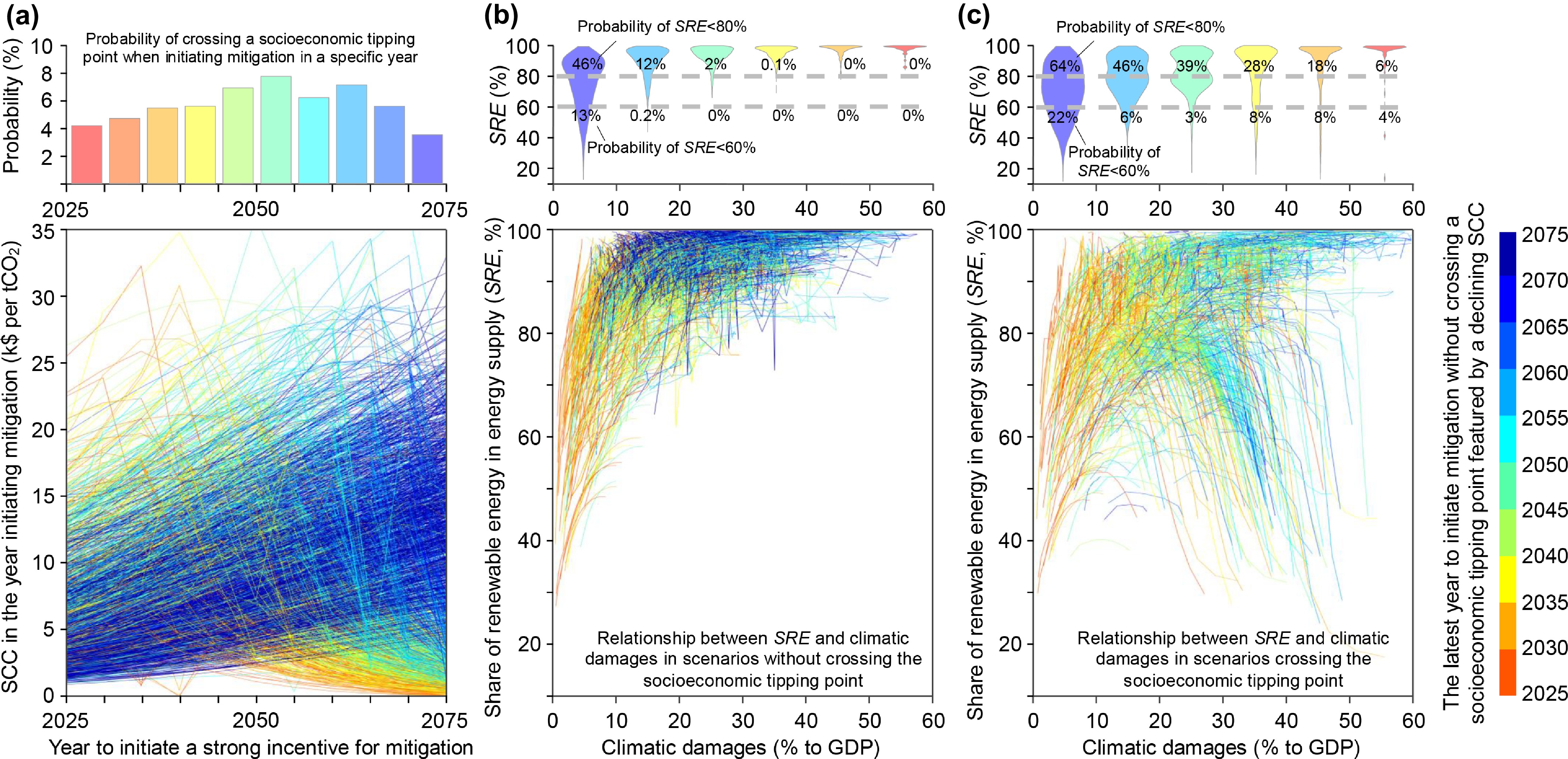
Figure 6.

Relationships between the share of renewable energy within total energy (SRE) and the projected climatic damage. (a) Comparison of the trend in the SCC estimated for the year of initiating a strong incentive for mitigation across 10,000 Monte Carlo simulations. The line color denotes the latest year of initiating a strong incentive for mitigation without crossing a socioeconomic tipping point featured by a declining SCC in the Monte Carlo simulations. The bar plot shows the probability of crossing this tipping point when mitigation is initiated within a 5-year period. (b) Relationship between SRE and climatic damage in scenarios without crossing a socioeconomic tipping point. (c) Relationship between SRE and climatic damage in scenarios crossing the socioeconomic tipping point featured by a declining SCC. In (b) and (c), the violin plot shows the probability of SRE based on the range of climatic damage in a future year.