-
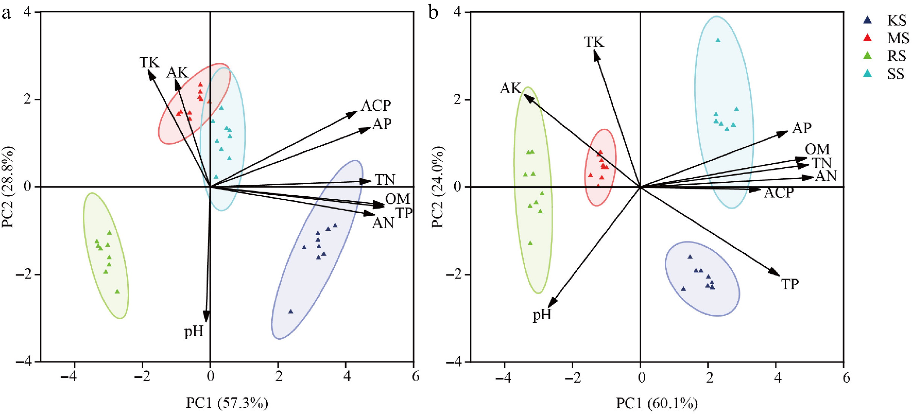
Figure 1.
Diversity differences among four soil conditions. (a) Pre-treatment. (b) Post-treatment. The different colored circles in the diagram represent different soil types; TN, total nitrogen; TP, total phosphorus; TK, total potassium; AN, acute nitrogen; AP, available phosphorus; AK, acute potassium; OM, organic matter; ACP, acid phosphatase; pH, acidity and alkalinity.
-

Figure 2.
Expression values of traits and contribution rates of variation sources under various soil conditions. Box plots indicate variability in plant height, biomass, and root metrics, and dots indicate individual data, p values represent overall differences between groups, the horizontal lines represent comparisons between the two groups at either end of the scale, * indicates the level of significance of differences obtained by two-by-two comparisons; H, Plant Height; ADW, Aboveground dry weight; LDW, Leaf dry weight; BDW, Branch dry weight; SDW, Stem dry weight; RDW, Root dry weight; SRL, Specific root length; SRA, Specific root area; RAD, Root average diameter; RBS, Root branching strength; TRL, Fine root length; TRA, Fine root surface area; TRV, Fine root volume; R/S, Root to shoot ratio; The ternary plot represents the share of genetic variance components, environmental variance components, and variance components of genotype-environment interactions for each of these metrics, with dots of the same color indicating replicate values for that metric. * p < 0.05; ** p < 0.01; *** p < 0.001.
-

Figure 3.
Plot of rank order effects of different family among soil environments. (a), (b), and (c) Representative differentiability and representativeness based on aboveground biomass, root biomass and plant height traits; Where the line with the arrow is the Average Environment Axis (AEA), through the connection between the average environment (the circle in front of the arrow) and the center point. The angle between the line segment of a test point and the Average Environment Axis is a measure of its representativeness of the target environment; the smaller the angle, the more representative it is, and the longer the line segment, the stronger the discriminatory power. If the angle between a test point and the mean environment axis is obtuse, it is not suitable as a test point. The direction of the arrow on the mean environmental axis is an evaluation of both the discriminatory power and representativeness of the test site. (d), (e), and (f) representative stable lineage ranking map based on plant height, aboveground biomass and root biomass traits. The high-yield and stable-yield performance plot requires an Environmental Mean Axis (EMA) represented by a straight arrowed line, as well as Mean Environmental Values (MEV) indicated by circles on the EMA. Additionally, a perpendicular line passing through the origin and orthogonal to the EMA is included. Each variety point is projected onto the EMA using a perpendicular line. The direction of the EMA indicates the approximate average yield trend of the varieties across all environments. The perpendicular line passing through the origin and orthogonal to the EMA represents the tendency of genotype-by-environment interactions (G × E). The longer the perpendicular line between a variety point and the EMA, the less stable the variety is. The numbers in the plot represent different varieties.
-
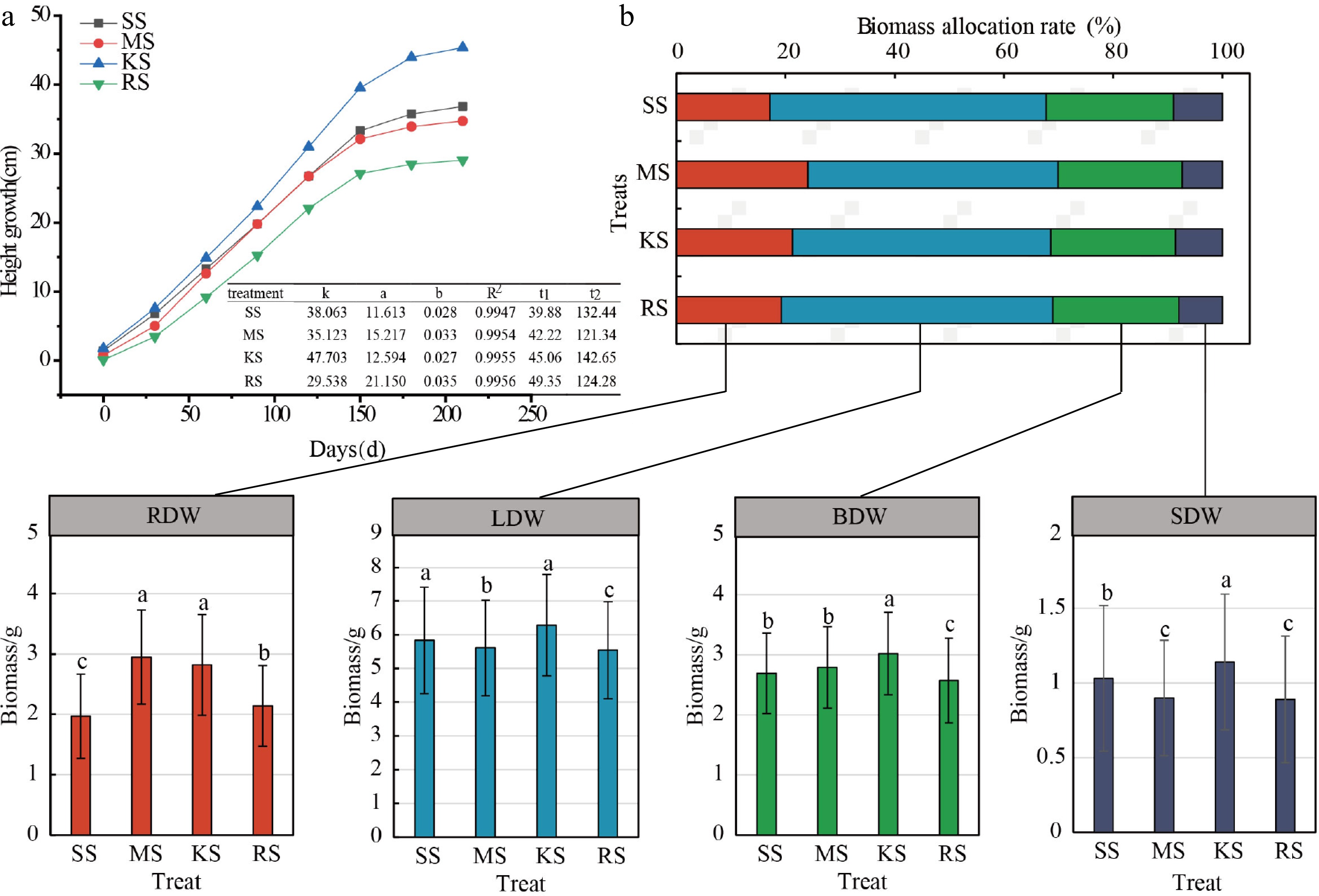
Figure 4.
Plant height growth curve and biomass allocation of cedar under different soil treatments. (a) Growth rhythm map, where k is the theoretical limit value of the upper limit value of the growth, and a and b are the coefficients to be determined, R2: coefficient of determination represents the goodness of fit of the model, reflecting the extent to which the independent variable explains the variation in the dependent variable.t1: the start time of the rapid growth period; t2: end of rapid growth period. (b) Biomass distribution graph. The horizontally arranged bar chart represents the biomass allocation proportions among root, stem, trunk, and leaf organs, while the vertically arranged bar chart indicates the variation in biomass measurements of each organ across treatments; Different lowercase letters denote significant differences between treatments. ADW: Aboveground dry weight; LDW: Leaf dry weight; BDW: Branch dry weight; SDW: Stem dry weight; RDW: Root dry weight.
-

Figure 5.
Distribution ratio and growth of D1–D5 radial root classes. (a) Proportion of root length grading (%). (b) Proportion of root surface area grading (%). (c) Proportion of root volume grading (%). (d) Root length. (e) Root surface. (f) Root volume. D1–D5 represent diameter levels, D1: 0 to 0.5 mm, D2: 0.5 to 1.0 mm, D3: 1.0 to 1.5 mm, D4: 1.5 to 2.0 mm, D5: > 2.0 mm.
-
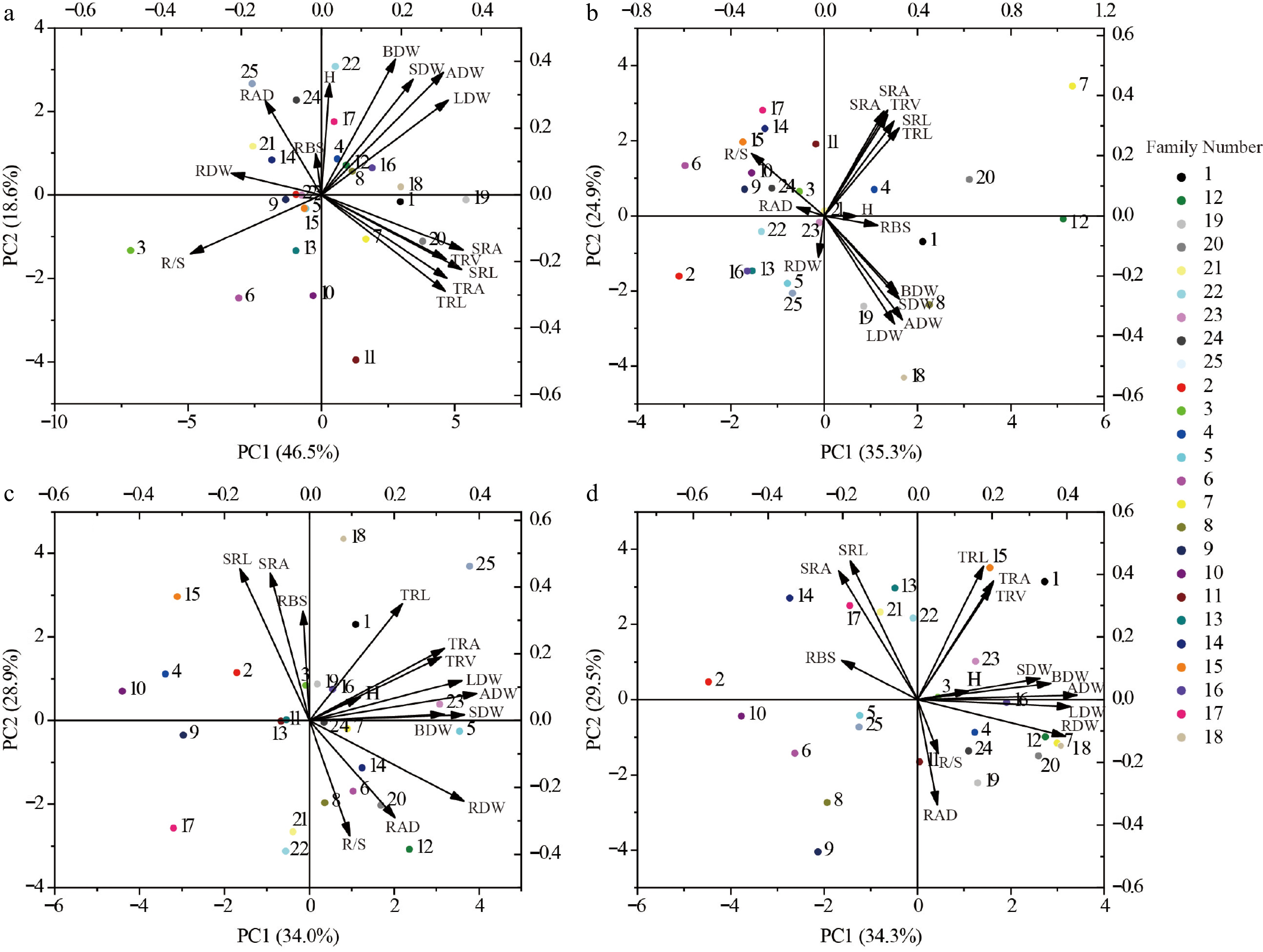
Figure 6.
Selection of different genotypes for growth in each of the four soils. (a) SS Soil conditions. (b) MS Soil conditions. (c) KS Soil conditions. (d) RS Soil conditions. The numbered points in the diagram represent different families of Chinese fir. H, Plant height; ADW, Aboveground dry weight; LDW, Leaf dry weight; BDW, Branch dry weight; SDW, Stem dry weight; RDW, Root dry weight; SRL, Specific root length; SRA, Specific root area; RAD, Root average diameter; RBS, Root branching strength; TRL, Fine root length; TRA, Fine root surface area; TRV, Fine root volume; R/S, Root to shoot ratio. Different colored circles represent different family.
-
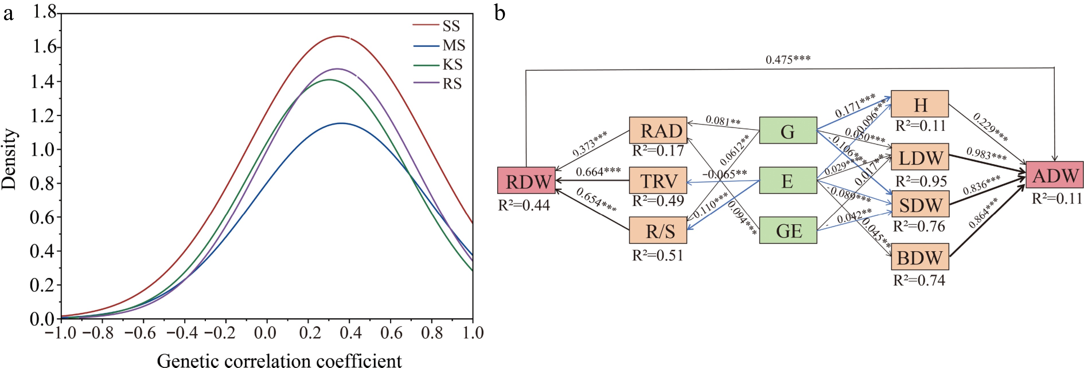
Figure 7.
(a) Frequency distribution of genetic correlation indices between all traits. The frequency of distribution of correlation coefficients, measured as genetic correlation coefficients between two indices, was calculated 91 times using 14 traits. (b) Partial least squares structural equation modeling (PLS-SEM) reveals direct and indirect effects of genotype and environment on growth and root function traits. AIC = 36.18, Fisher's C = 41, p = 0.072 in the model, Solid blue arrows indicate negative paths (p < 0.05), solid black arrows indicate positive paths (p < 0.05), and the width of the arrows indicates the strength of the causal relationship. Numbers on the line adjacent to the arrows are standardized path coefficients. R2 indicates the total variance explained by the model. H, Plant Height; ADW, Aboveground dry weight; LDW, Leaf dry weight; BDW, Branch dry weight; SDW, Stem dry weight; RDW, Root dry weight; RAD, Root average diameter; TRV, Fine root volume; R/S, Root to shoot ratio; * p < 0.05; ** p < 0.01; *** p < 0.001.
-
Traits Mean value F value Coefficient of variation (%) hf2 G E G × E CVg CVe H/cm 51.86 9.75** 144.99** 4.18** 3.58 9.10 0.57 ADW/g 9.57 4.79** 17.45** 1.91** 6.56 23.25 0.60 LDW/g 5.81 4.92** 13.16** 1.84** 6.91 23.61 0.63 BDW/g 0.99 5.90** 19.94** 1.66** 13.92 40.78 0.72 SDW/g 2.77 5.76** 21.77** 2.54** 6.66 22.11 0.56 RDW/g 2.47 1.27** 103.99** 2.22** 4.69 28.80 0.30 SRL/(cm/g) 1,030.05 4.38** 30.54** 6.54** 5.85 23.90 0.25 SRA/(cm2/g) 179.50 5.84** 23.90** 7.54** 3.87 17.81 0.18 RAD/mm 2.53 3.69** 37.35** 6.06** 2.73 16.15 0.11 RBS 8.75 21.68** 66.12** 29.46** 7.20 15.50 0.21 TRL/cm 2,338.59 3.35** 63.00** 3.30** 0.91 24.69 0.10 TRA/cm2 331.90 3.36** 80.14** 2.60** 3.60 24.86 0.23 TRV/cm3 6.04 4.07** 80.57** 2.77** 4.91 25.87 0.32 R/S 0.26 3.75** 163.74** 4.82** 3.88 21.07 0.23 H, Plant Height; ADW, Aboveground dry weight; LDW, Leaf dry weight; BDW, Branch dry weight; SDW, Stem dry weight; RDW, Root dry weight; SRL, Specific root length; SRA, Specific root area; RAD, Root average diameter; RBS, Root branching strength; TRL, Fine root length; TRA, Fine root surface area; TRV, Fine root volume; R/S, Root to shoot ratio. G, Genotype interactions; E, Environment interactions; G × E, Genotype and environment interactions; CVg, Genetic variation coefficient; CVe, Environment variation coefficient; hf2, Family heritability. ** indicates a significant difference at p < 0.01. Table 1.
ANOVA tests for growth and root traits of Chinese fir seedlings.
Figures
(7)
Tables
(1)