-
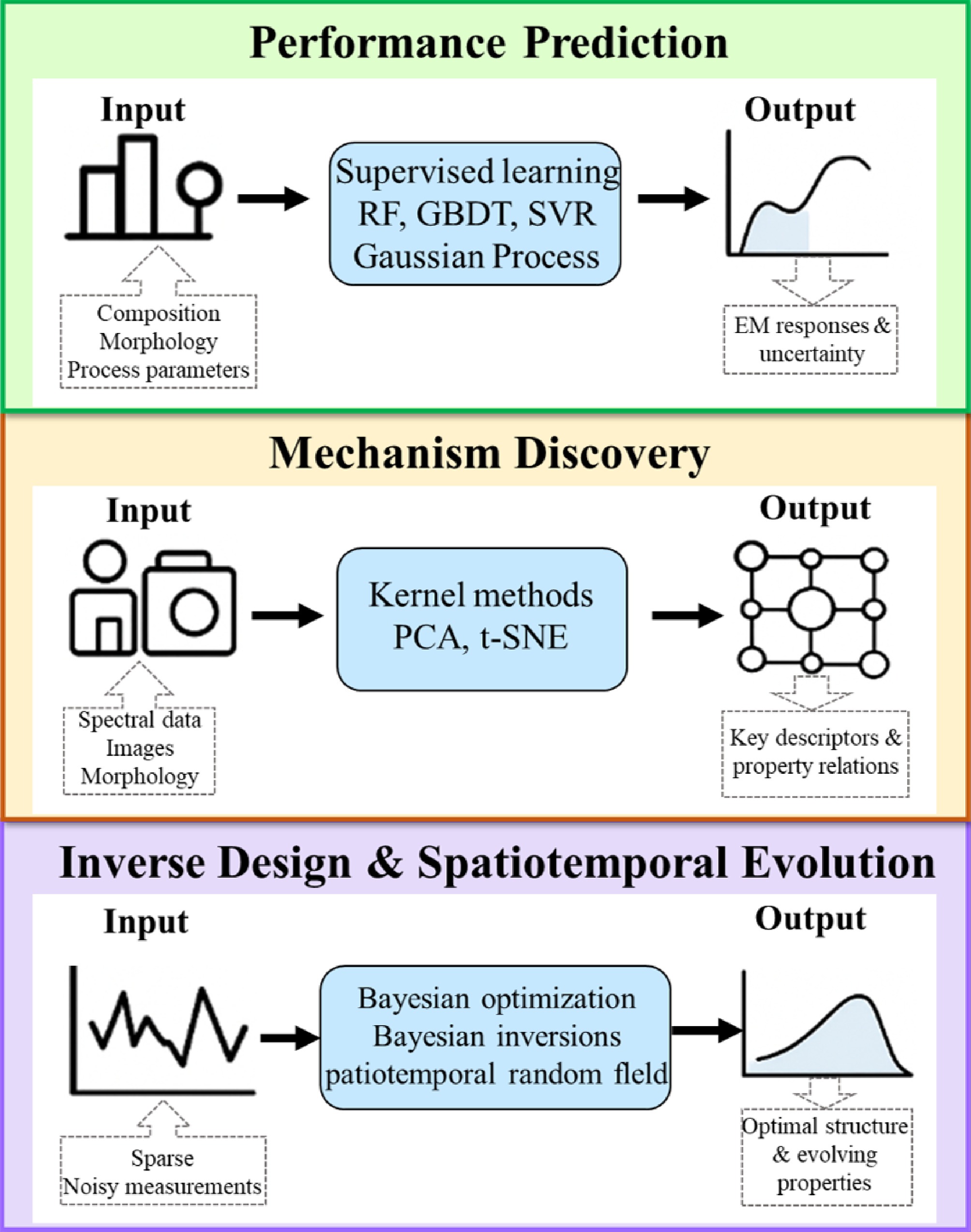
Figure 1.
Conceptual framework of statistical approaches in electromagnetic functional materials.
-
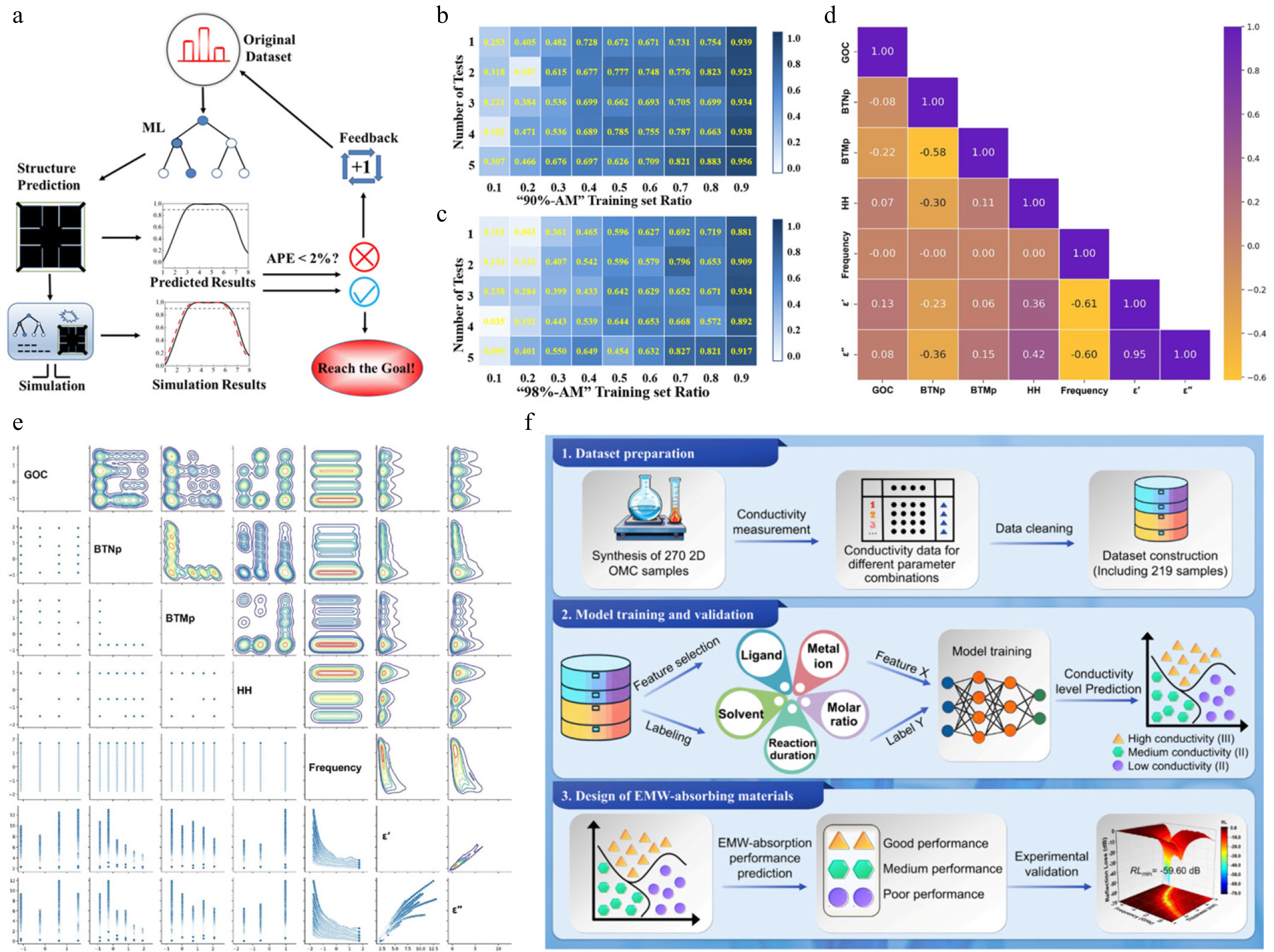
Figure 2.
(a) Schematic illustration of the machine learning–assisted prediction workflow for optimizing metasurface structural parameters. (b), (c) Coefficients of determination (R2) under varying training set proportions[11]. (d) Heat map of Pearson correlation coefficients between input features and output variables. (e) Correlation matrix of input features with dielectric properties, visualized through scatterplots. Diagonals show feature distributions[55]. (f) Machine learning strategy for conductivity prediction and electromagnetic wave absorber design in 2D ordered mesoporous carbons (OMCs)[12].
-
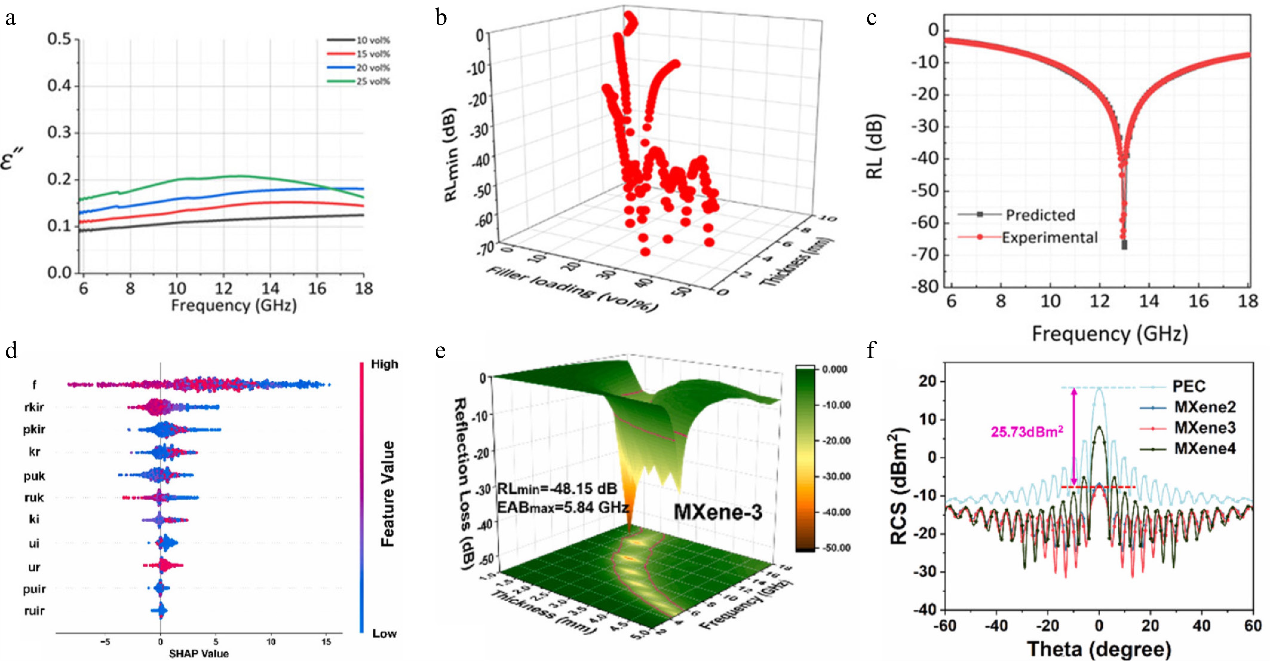
Figure 3.
(a) Measured dielectric permittivity of Fe2O3-loaded PDMS nanocomposites[57]. (b) Predicted minimum reflection loss (RLmin) of PDMS nanocomposites with varying Fe2O3 nanoparticle loadings (0.1–50 vol%) at their optimal thicknesses. (c) Comparison between predicted and experimentally measured reflection loss values[58]. (d) Relationship between feature variables and their SHAP values as computed by the regression model. (e) Three-dimensional plots of reflection loss for the MXene-3 sample. (f) Simulated radar cross-section (RCS) curves of bare PEC vs PEC coated with the absorbing layer[59].
-
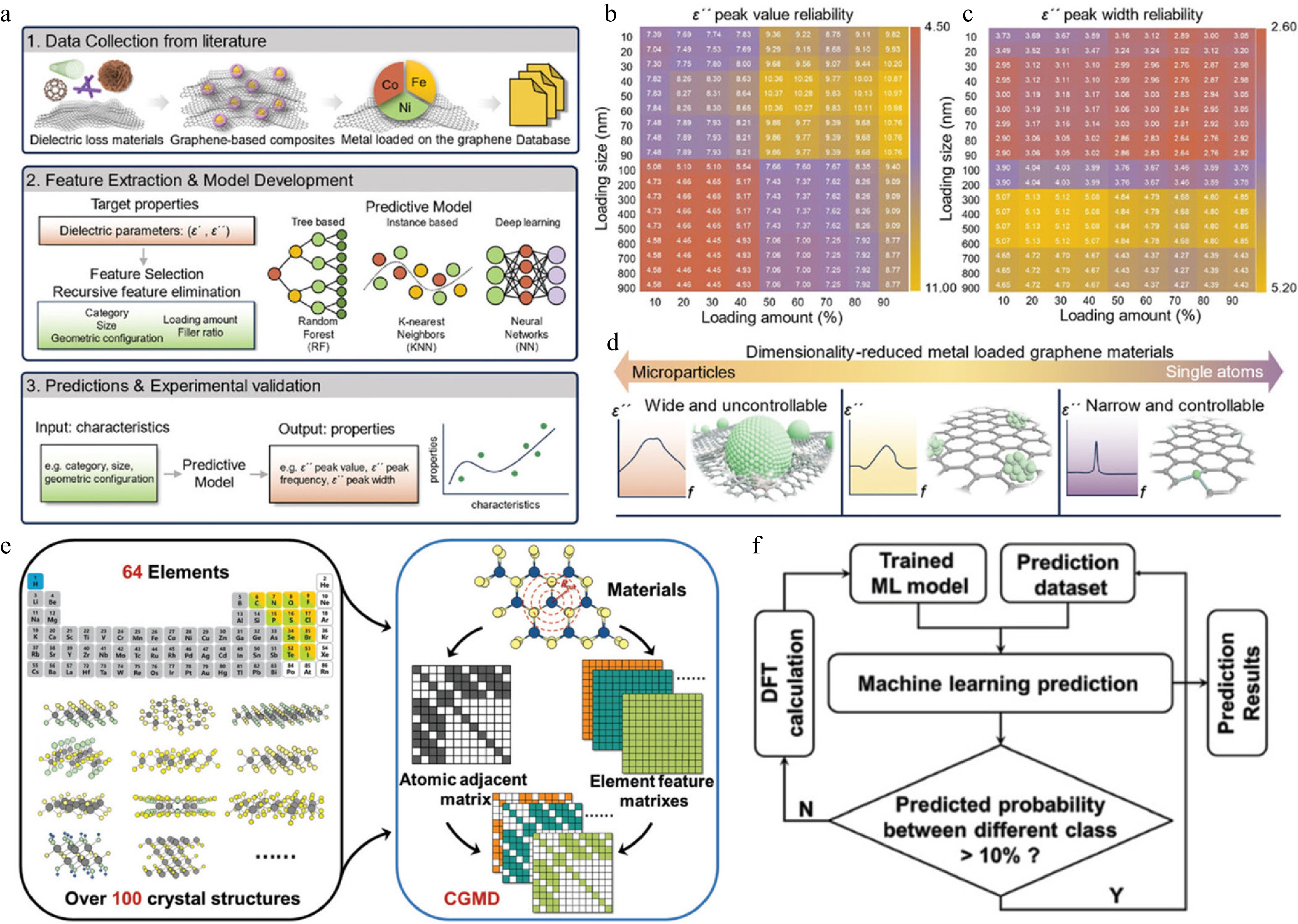
Figure 4.
(a) Workflow for predicting the relationship between material descriptors and dielectric loss parameters. (b) Reliability of ε peak values for Co/graphene composites at 50% loading. (c) Reliability of peak widths under the same condition. (d) Influence of metal loading size on dielectric loss parameters in graphene-based materials[5]. (e) Schematic of the Crystal Graph Multilayer Descriptor (CGMD) computation. (f) Iterative machine learning feedback loop for active materials discovery[61].
-
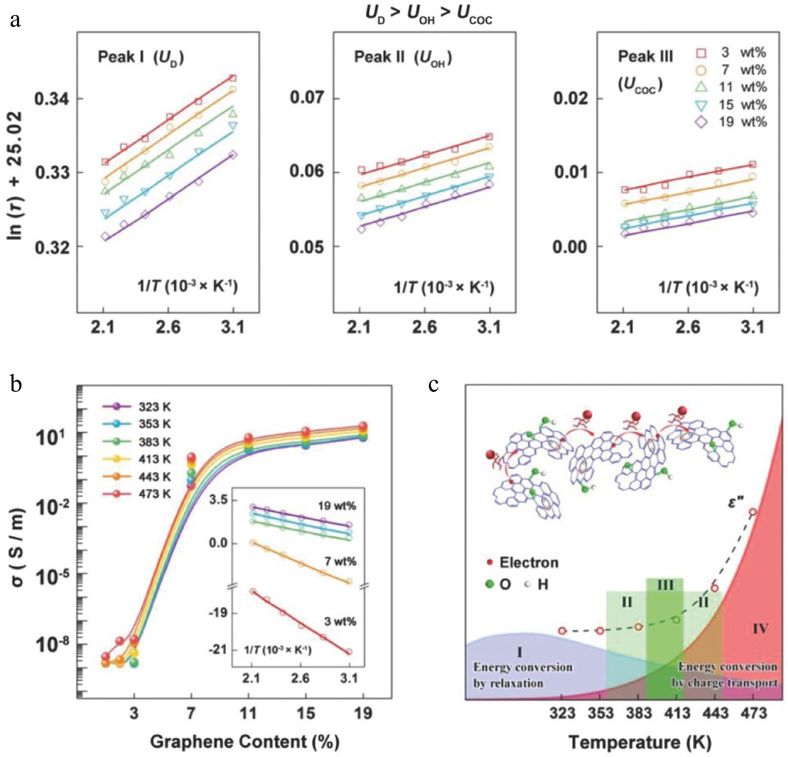
Figure 5.
(a) Arrhenius plots of ln(τ) vs inverse temperature (T−1) for relaxation peaks of different defect-induced dipoles. (b) Conductivity (σ) as a function of graphene content from 323 to 473 K (inset: ln(σ) vs T−1, where the charge transport barrier is proportional to the absolute slope). (c) Temperature dependence of polarization relaxation loss (εp″), and charge transport loss (εc"), with regions I−IV indicating: I—dominance of εp"; II—synergistic and competitive interaction between εp″ and εc″; III—equilibrium between εp" and εc"; IV—dominance of εc"[64].
-
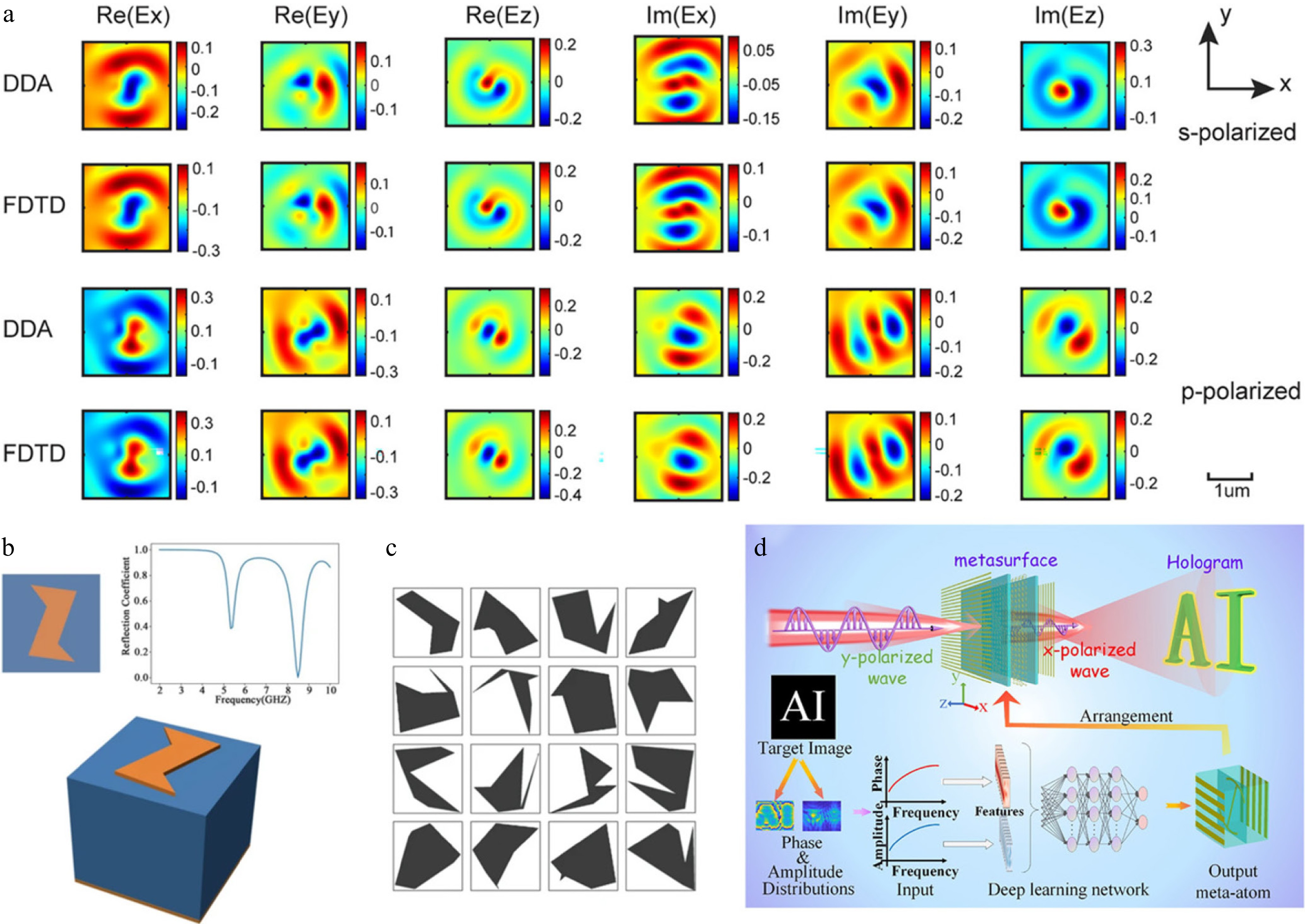
Figure 6.
(a) Convergence of 1D cylindrical Green's function discrete dipole approximation (DDA) results validated against finite-difference time-domain (FDTD) simulations. Real and imaginary components of the electric field computed by both methods for a larger gold elliptic cylinder at discretization factor D = 3[68]. (b) A sample of data consisting of a 2D cross-sectional image of a structural design and the corresponding conversion efficiency as an optical response[71]. (c) Example of a random polygon dataset for CGAN training[71]. (d) Schematic diagram of the deep learning network empowered metasurface hologram inverse design via the simultaneous control of phase and amplitude[72].
Figures
(6)
Tables
(0)