-
-
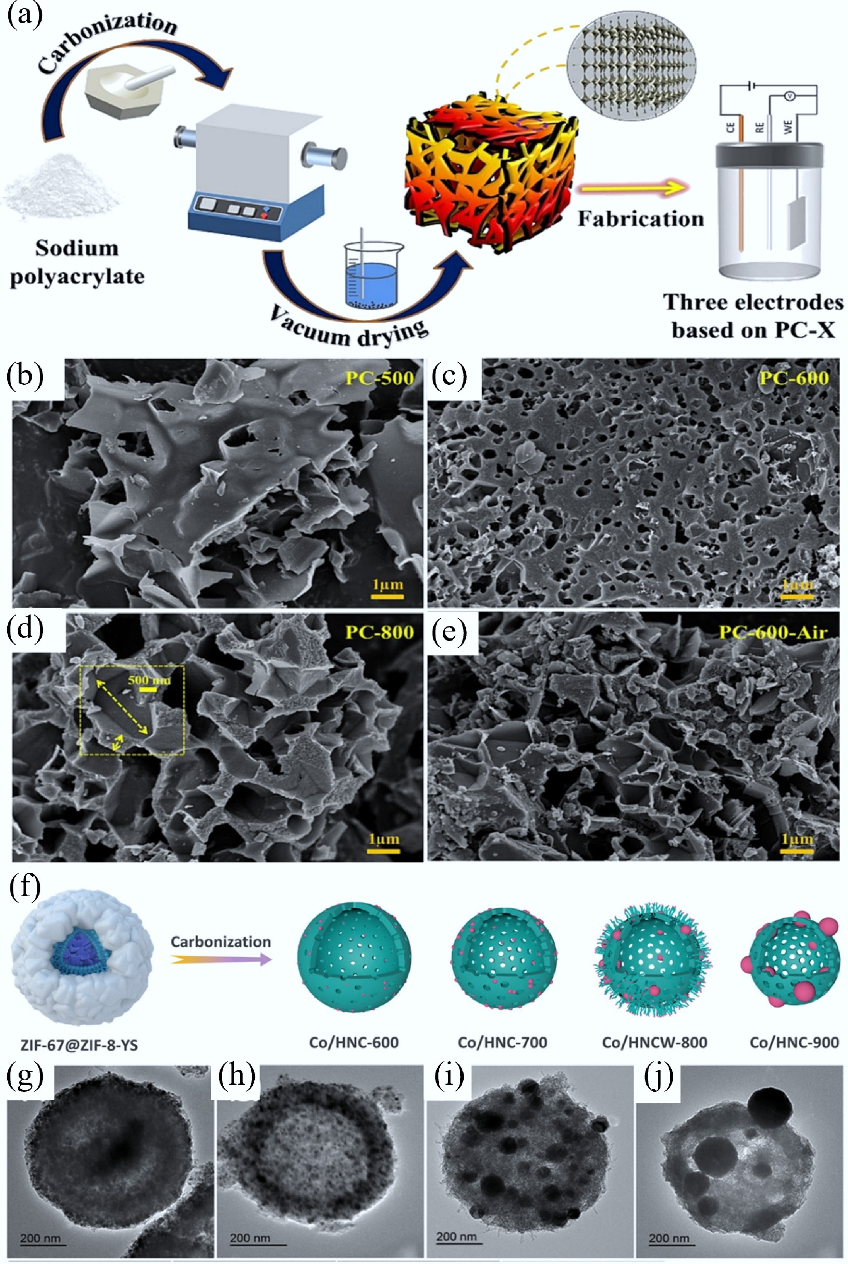
Figure 2.
(a) Synthesis process of sodium polyacrylate-based PC. SEM graphs of PC carbonized at (b) 500 °C, (c) 600 °C, and (d) 800 °C in an Ar atmosphere, and (e) PC-600 fabricated in air[29]. (f) Diagram of Co/HNC-x samples (where x denotes calcination temperatures: 600, 700, 800, and 900 °C), prepared by carbonizing the ZIF-67@ZIF-8-YS precursor for 2 h in N2, and the corresponding TEM images of (g) Co/HNC-600, (h) Co/HNC-700, (i) Co/HNCW-800, and (j) Co/HNC-900[46].
-
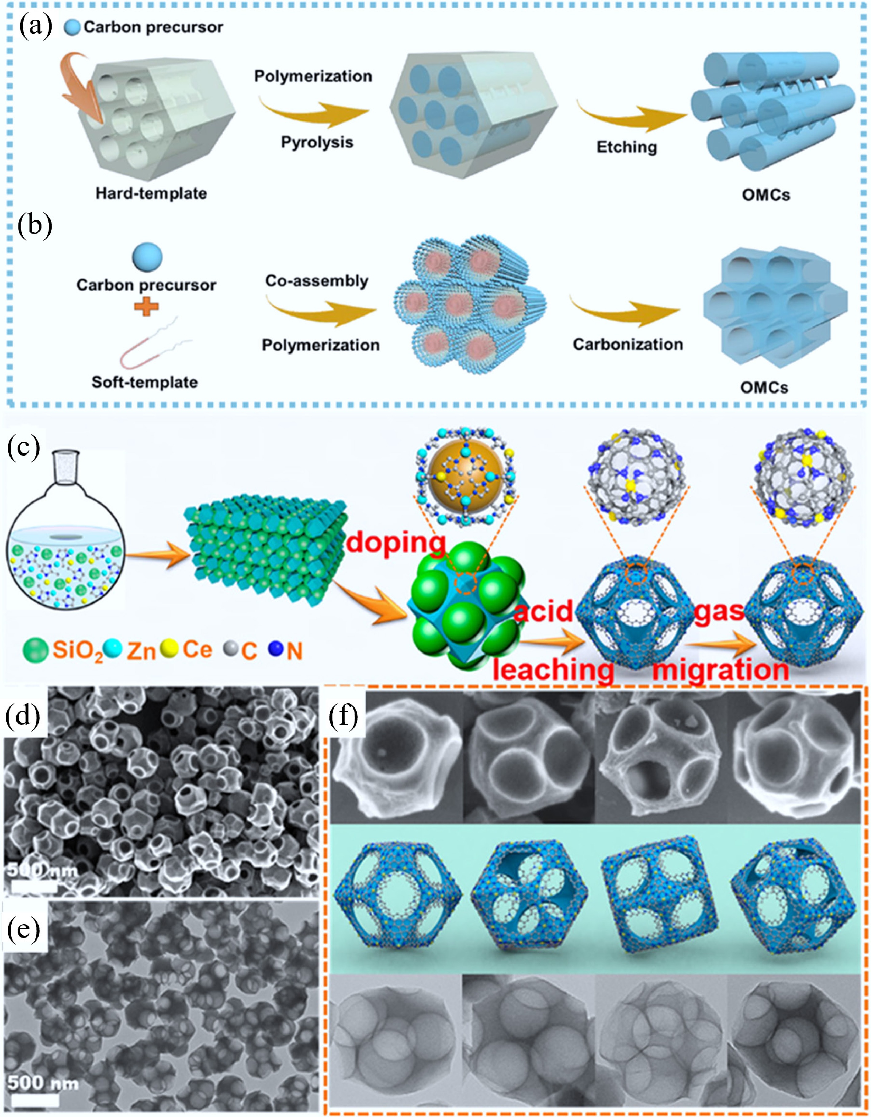
Figure 3.
Scheme for the synthesis of OMCs by using (a) ordered mesoporous silicates as hard-templates and (b) supramolecular aggregates as soft-templates[30]. (c) Fabrication procedure of a hierarchically macro–meso–microporous N-doped carbon (Ce SAS/HPNC) catalyst by using SiO2 as hard-templates, (d) SEM, (e) TEM, and (f) both images of Ce SAS/HPNC corresponding to the models from different angles[49].
-
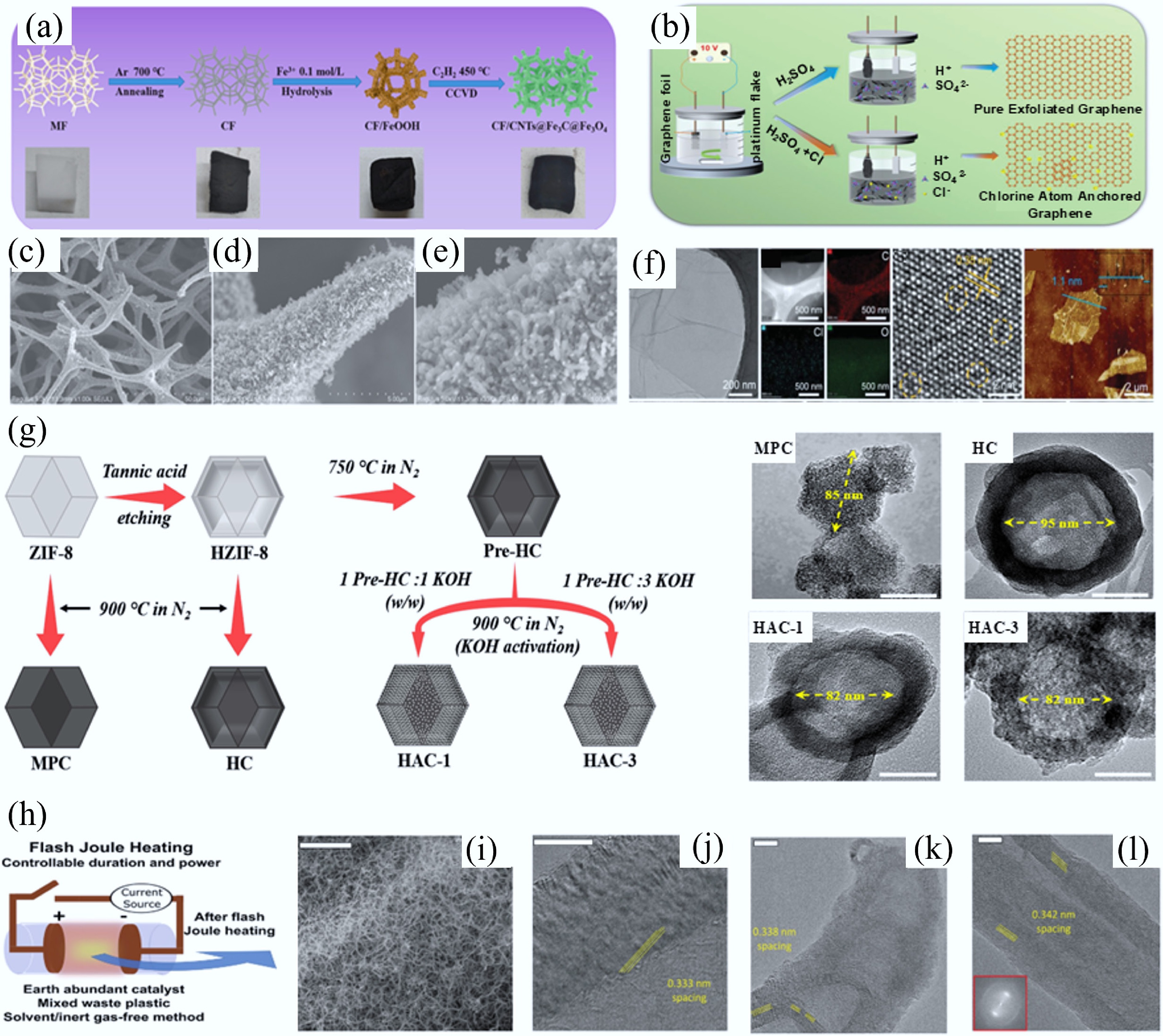
Figure 4.
(a) Synthesis of CF/CNTs@Fe3C@Fe3O4 via in-situ growth of CNTs via catalytic CVD of C2H2 at 450 °C. (b)–(d) SEM images of CF/CNTs@Fe3C@Fe3O4 with different magnifications[57]. (e) Preparation process of chlorine-doped graphene (working electrode: graphite flake; counter electrode: platinum foil; electrolyte: sulfuric acid with chloride salt; applied potential: +10 V) and (f) morphology and structure characterizations[62]. (g) Synthetic pathways and corresponding morphologies of MPC (microporous carbon from ZIF-8 carbonization), HC (hollow carbon from tannic acid-etched ZIF-8 carbonization), HAC-1 and HAC-3 (hollow AC from HC activated with KOH/pre-HC weight ratios of 1 and 3, respectively, at 900 °C in N2)[63]. (h) Preparation of flash 1D materials via FJH using waste polymer as starting material (~3,000 K temperatures generated in 0.05–3 s) and (i)−(l) different morphologies of flash 1D materials[64].
-
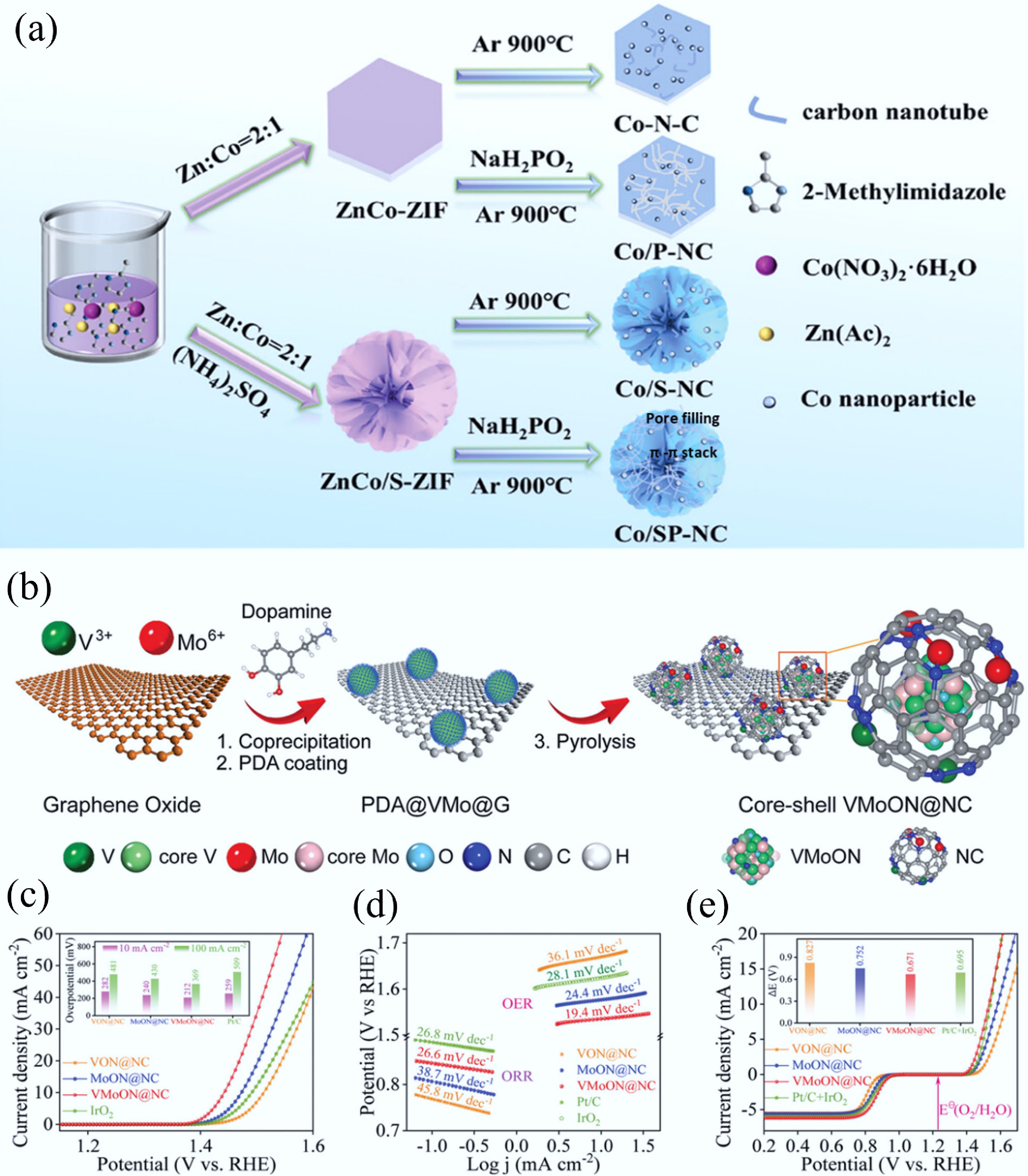
Figure 5.
(a) The preparation process of 3D N/P/S-tri-doped nanoflower with highly branched CNTs bifunctional catalyst[34]. (b) The preparation of the core–shell VMoON@NC 3D electrode architecture. (c) OER polarization curves of the as-obtained catalysts. (d) Tafel plots for ORR and OER catalysts. (e) Overall polarization curves within the ORR and OER potential window of the Mo SACs[33].
-
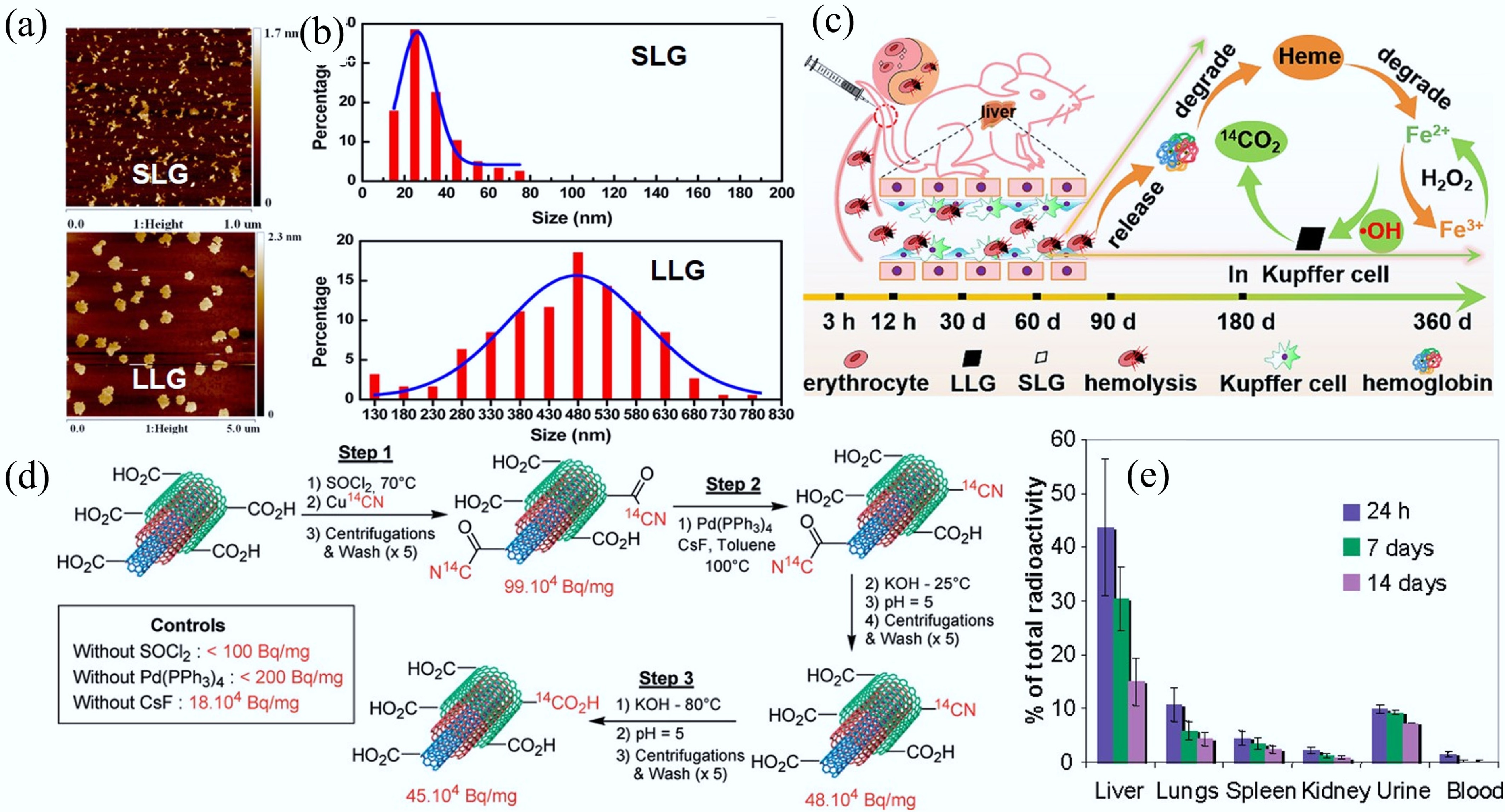
Figure 6.
(a) Representative atomic force microscope topography of SLG and LLG. (b) Histogram of SLG and LLG size distribution. (c) Schematic illustration of the process of LLG triggering the Fenton reaction in Kupffer cells[85]. (d) Preparation process of 14C-labelled multi-walled CNTs. (e) Biodistribution of intravenously administered 14C-labeled multi-walled CNTs at different time points after exposure. Each group contained six animals (n = 6)[88].
-
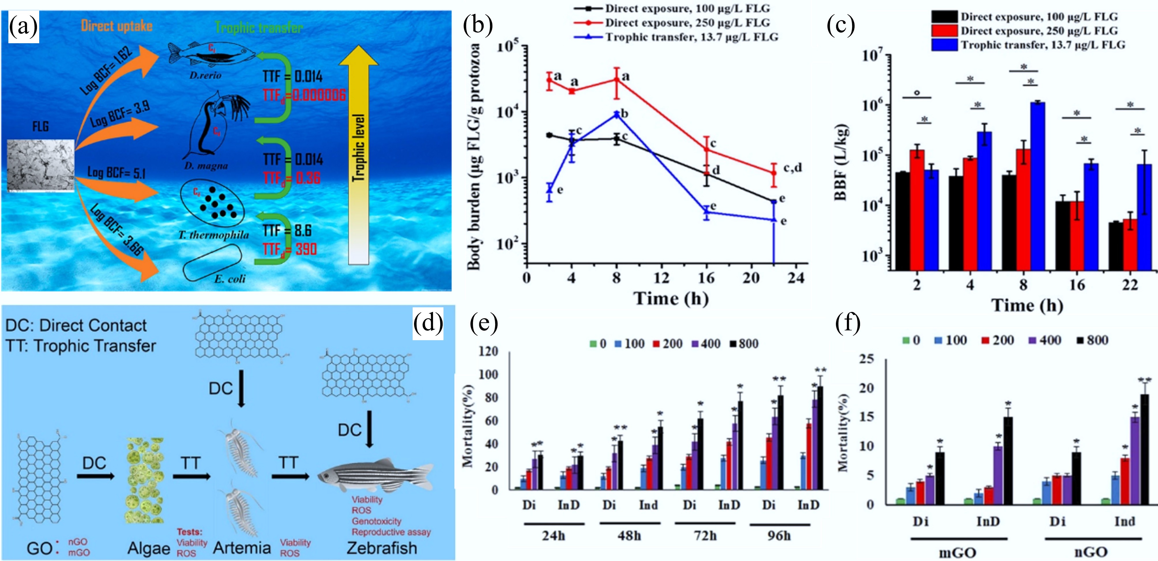
Figure 7.
(a) Schematic diagram of the bioaccumulation of 14C-labeled few-layer graphene (FLG) in an aquatic food chain through direct uptake or trophic transfer. (b) Body burden of T. thermophile during the direct exposure to FLG with concentration of 100 or 250 μg/L and trophic transfer from FLG associated E. coli. Each data point represents the mean of three independent replicates, with error bars showing the standard deviation (SD). Statistical significance is determined using Tukey's multiple comparison test. Groups labeled with the same letter do not differ significantly (p ≥ 0.05). (c) BBFs of FLG at different time points during T. thermophila growth in the presence of FLG, administered either directly in the medium (direct exposure) or with FLG-encrusted E. coli (trophic transfer). Bars represent BBFs derived from the mean values of FLG measured in triplicate. Asterisks (*) denote statistically significant differences[31]. (d) Schematic diagram of direct contact and trophic transfer of GO nanosheets in an aquatic food chain. (e) Mortality of Artemia salina caused by Nano-GO. (f) Mortality of D. rerio caused by Micro-GO and Nano-GO (in the Figures, direct ingestion and trophic transfer pathways are denoted as Di and InD, respectively). In (e) and (f), statistical significance is indicated by (*) and (**), corresponding to p ≤ 0.05 and p ≤ 0.01, respectively. All experiments were conducted in triplicate[106].
-
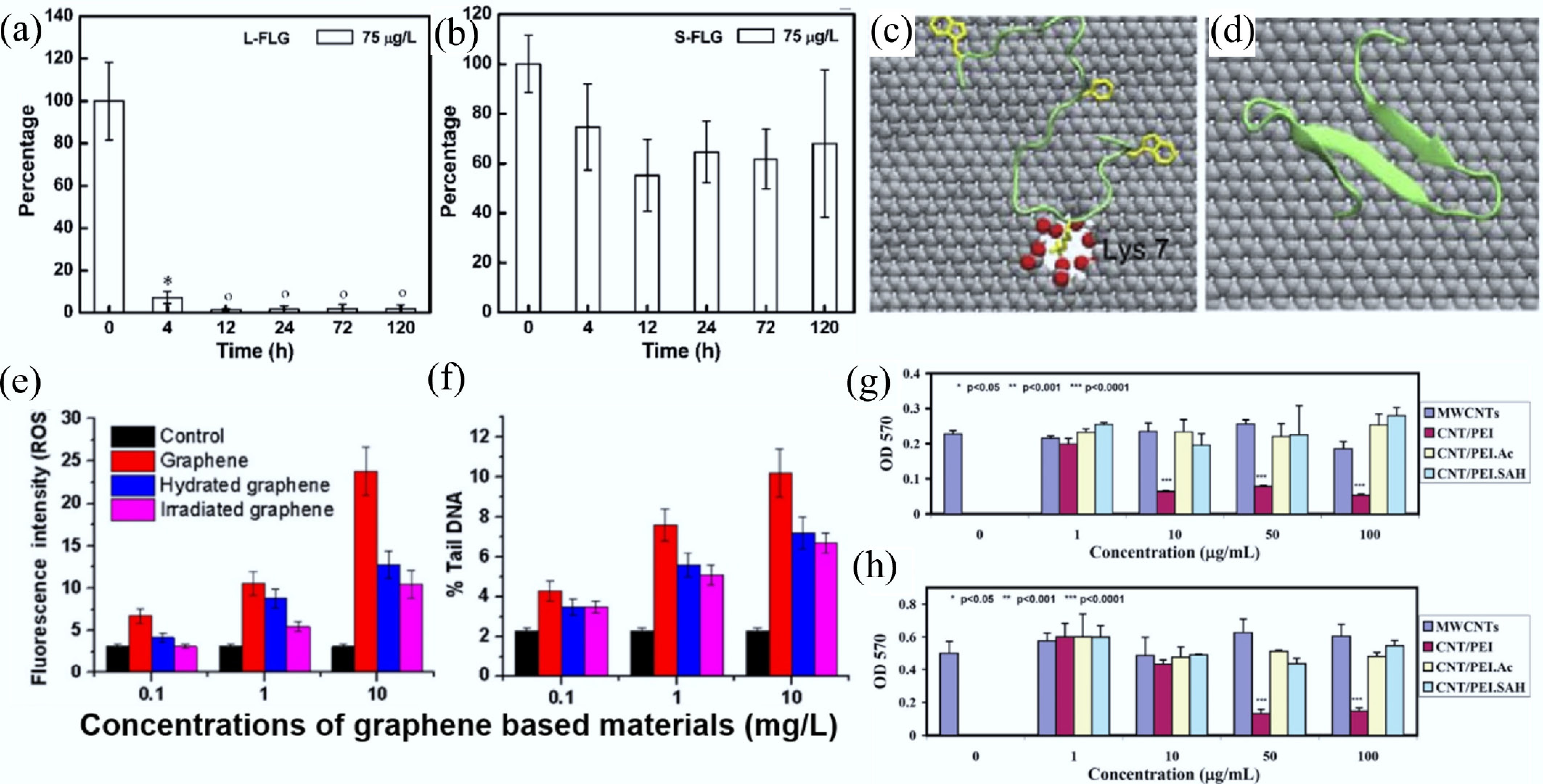
Figure 8.
Depuration of (a) Larger few-layer graphene and (b) Smaller few-layer graphene in zebrafish. Data are presented as mean ± SD (n = 5). Statistical significance was determined by Tukey's test (p < 0.05). Symbols (°) and (*) indicate values not significantly or significantly different from zero, respectively[90]. Representative contact configuration of YAP65WW protein adsorption onto (c) defective graphene and (d) ideal graphene surfaces (carbon, silver; oxygen, red; hydrogen, white). The critical residue Lys-7 involved in the binding process is labeled[114]. Effects of hydration and visible-light irradiation on the reduction of (e) oxidative stress and (f) DNA damage induced by pristine graphene. All experiments were conducted in triplicate, and error bars represent mean ± SD[101]. MTT assay results of cell viability for (g) FRO (a human thyroid cancer cell line) and (h) KB (a human epithelial carcinoma cell line) after 24 h treatment with differently functionalized MWCNTs. Each treatment was performed in triplicate, and error bars represent mean ± SD. Statistical significance was determined using the ANOVA test and is indicated by (*), (**), and (***) for p < 0.05, p < 0.001, and p < 0.0001, respectively[123].
-
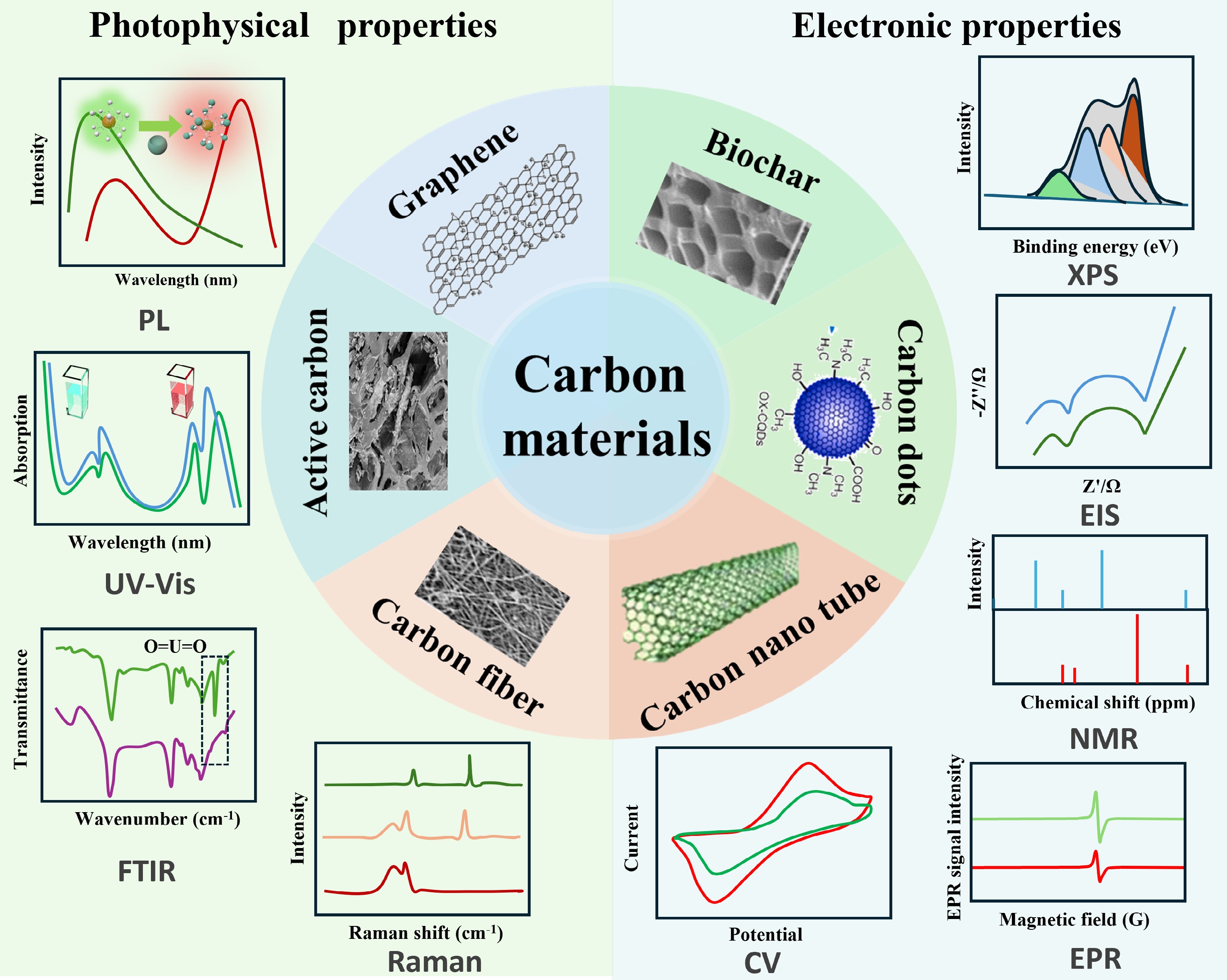
Figure 9.
Comprehensive analysis of structural characteristics and functional properties in sustainable CMs.
-
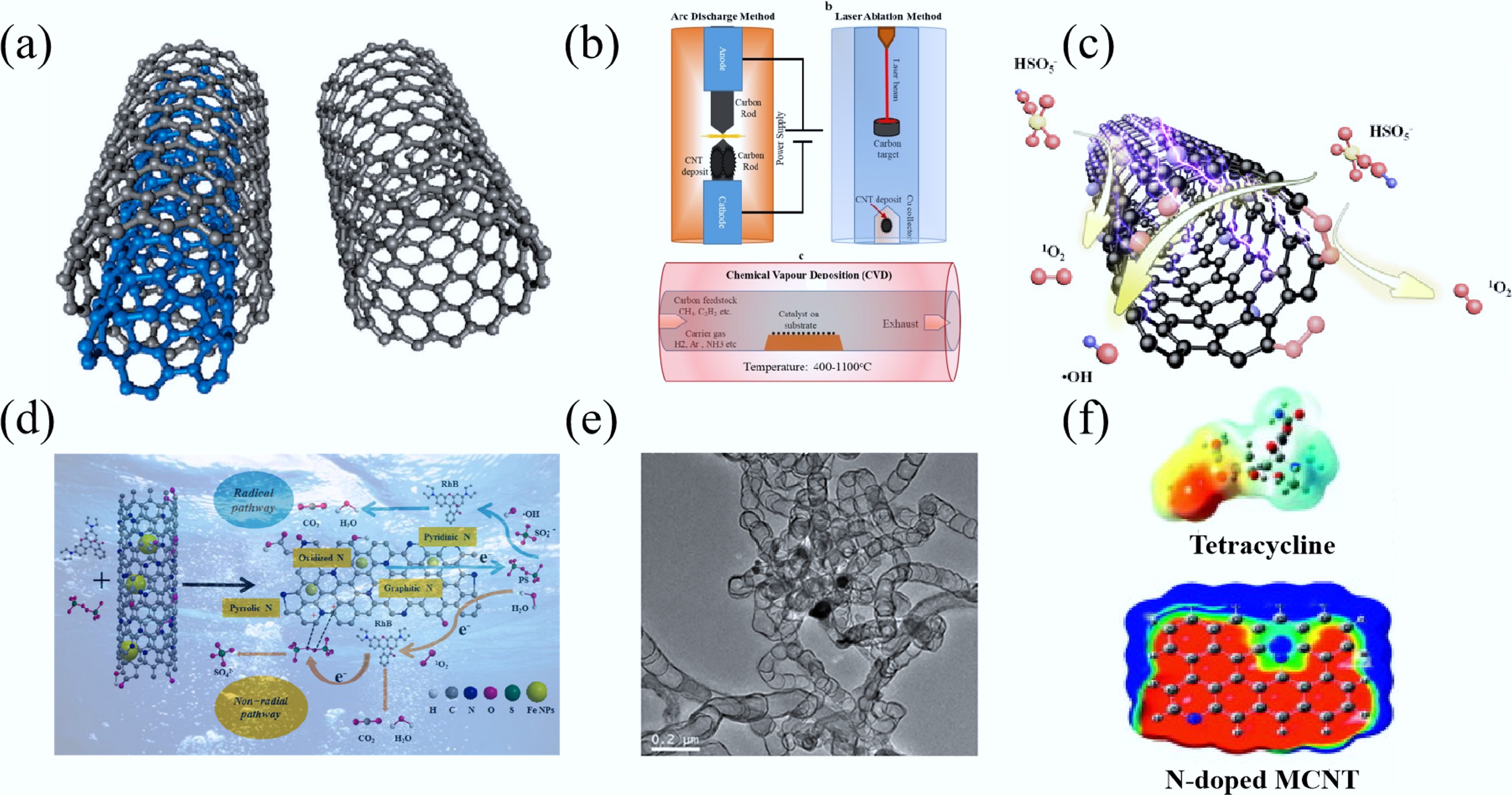
Figure 10.
(a) CNTs with different forms, monolithic (right) and multilayered CNTs (left)[270]. (b) Synthesis of CNTs[271]. (c) ROS generation mechanism based on the electrochemical nZVC-CNT/ peroxymonosulfate (PMS) filter[272]. (d) Schematic illustration of reaction mechanism for Rhodamine B (RhB) degradation by Fe@NCNT-BC-800/PS[273]. (e) TEM image of Fe@NCNT-BC-800[273]. (f) Electron density distribution of Tetraethylamine[274].
-
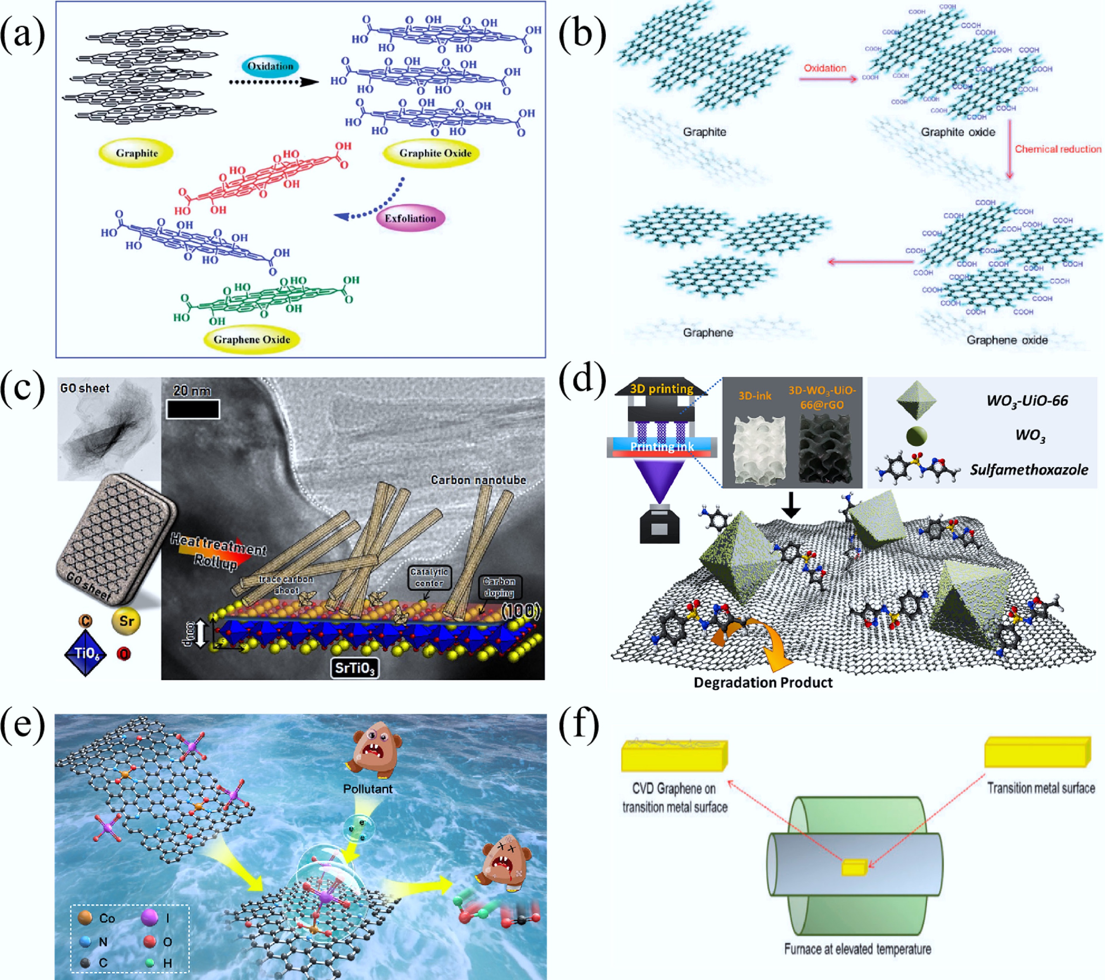
Figure 11.
(a) Production method of GO[285]. (b) Transformation pathway of graphite to GO and rGO[282]. (c) Schematic illustration of the formation of CNTs and carbon-doped SrTiO3 and its TEM image[286]. (d) Schematic illustration of sulfamethoxazole (SMX) degradation mechanism upon 3D-printed-WO3-UiO-66@rGO photocatalyst system[287]. (e) Mechanism of the 4-CP degradation upon N-rGO-CoSA[288]. (f) Graphene synthesis via the CVD method[282].
-
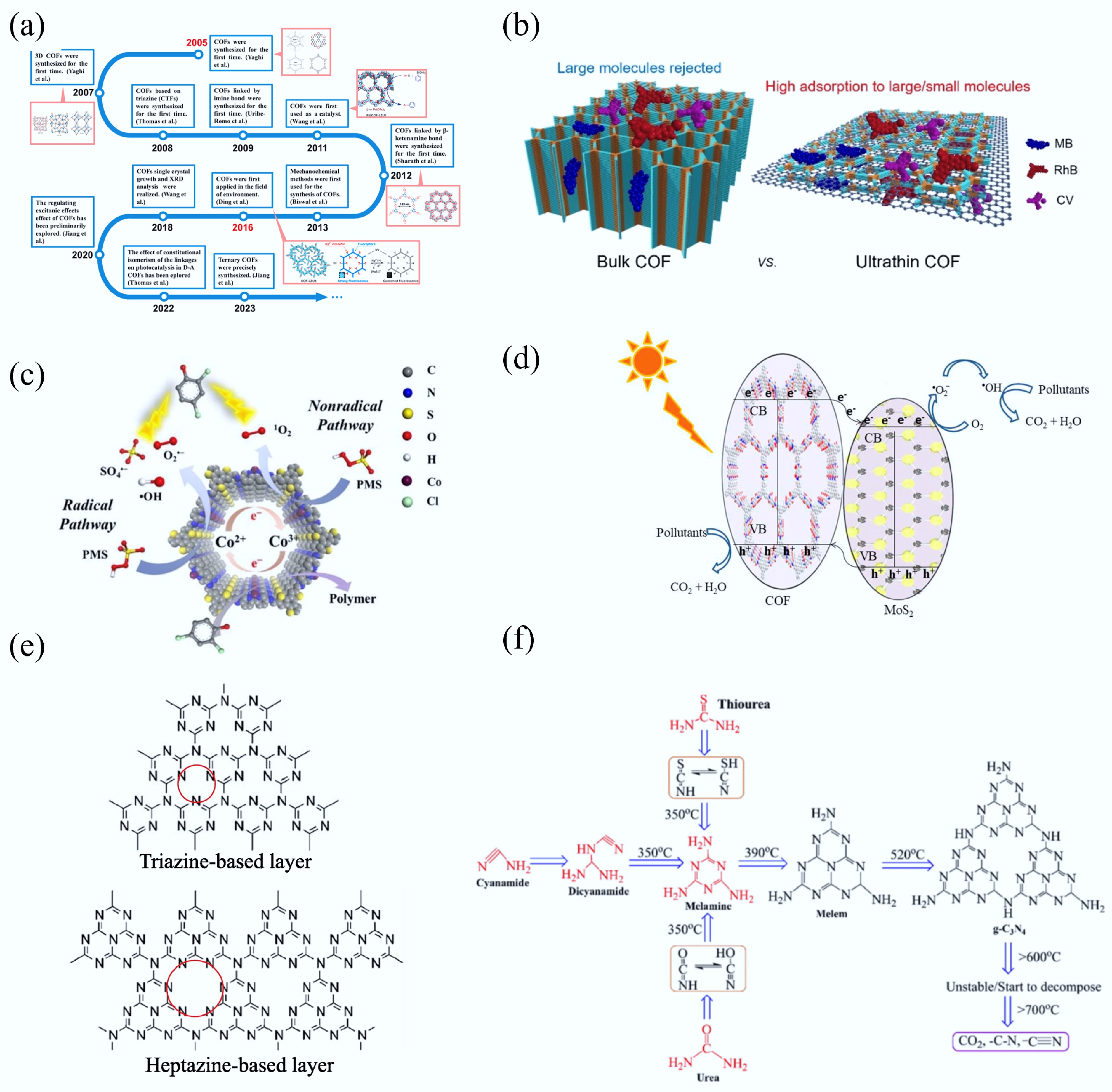
Figure 12.
(a) Development procedure of COFs[307]. (b) Schematic illustration of dye adsorption mechanism over bulk COF and ultrathin COF[308]. (c) Schematic illustration of 2,4-DCP mineralization mechanism over JLNU-317-Co/PMS[36]. (d) Schematic diagram of photocatalytic reaction mechanism over MoS2/COF[309]. (e) Layers description based on triazine and heptazine units[310]. (f) Schematic diagram of structure related to different precursors and pyrolysis temperature[311].
-
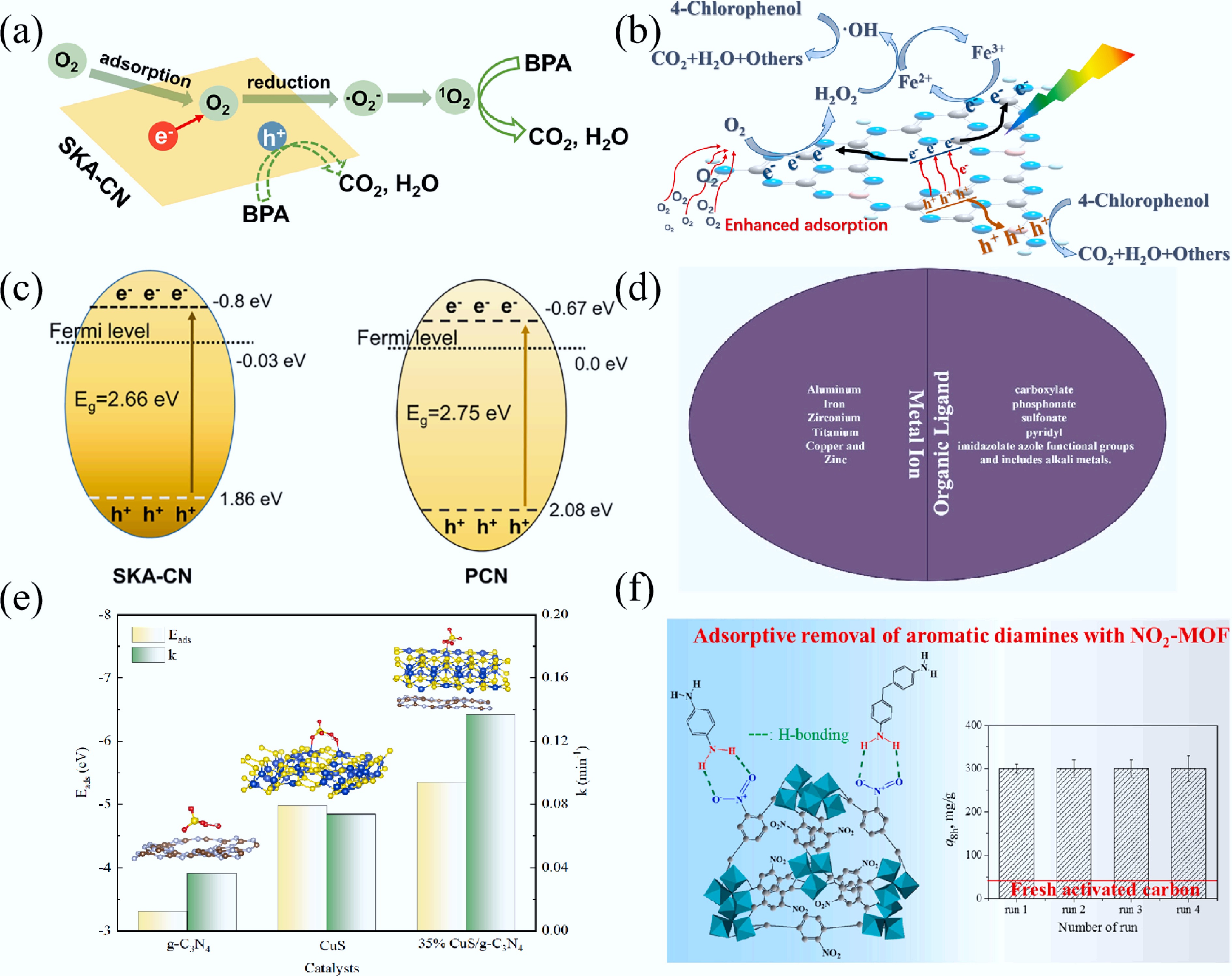
Figure 13.
(a) Schematic illustration of BPA degradation through 1O2 generated by SKA-CN[314]. (b) Schematic illustration of photocatalysis-self-Fenton degradation of 4-CP over Coral-B-CN[315]; (c) Band diagrams of SKA-CN and PCN[314]. (d) Composition of MOFs[316]. (e) Relationship between Eads and k (inset: geometric configurations for PMS adsorption on catalysts)[317]. (f) Illustration of the H-bonding between diamines and NO2-MOF and the recyclability[318].
-
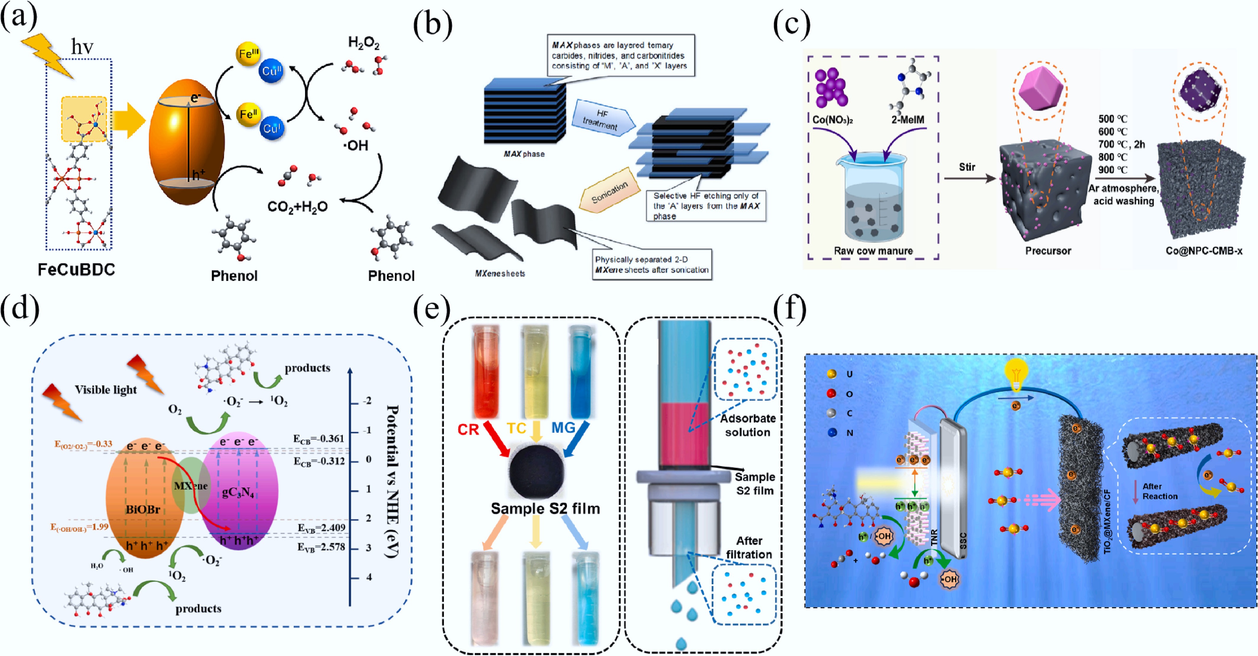
Figure 14.
(a) Schematic illustration of phenol degradation over FeCuBDC photo-Fenton system[327]. (b) The exfoliation of MAX phases and formation of MXenes[332]. (c) The schematic of the Co@NPC-CMB-x synthesis[328]. (d) Schematic illustration of charge transfer process on CBM for TCH degradation[333]. (e) Photographic image of sample S2 films for filtration of adsorbates and the schematic illustration of the filtering mechanism[334]. (f) Proposed mechanism of the self-driven solar coupling system (SSCS) for simultaneous uranyl ions (UO22+) reduction, organic pollutant oxidation and electricity production under sunlight[335].
-
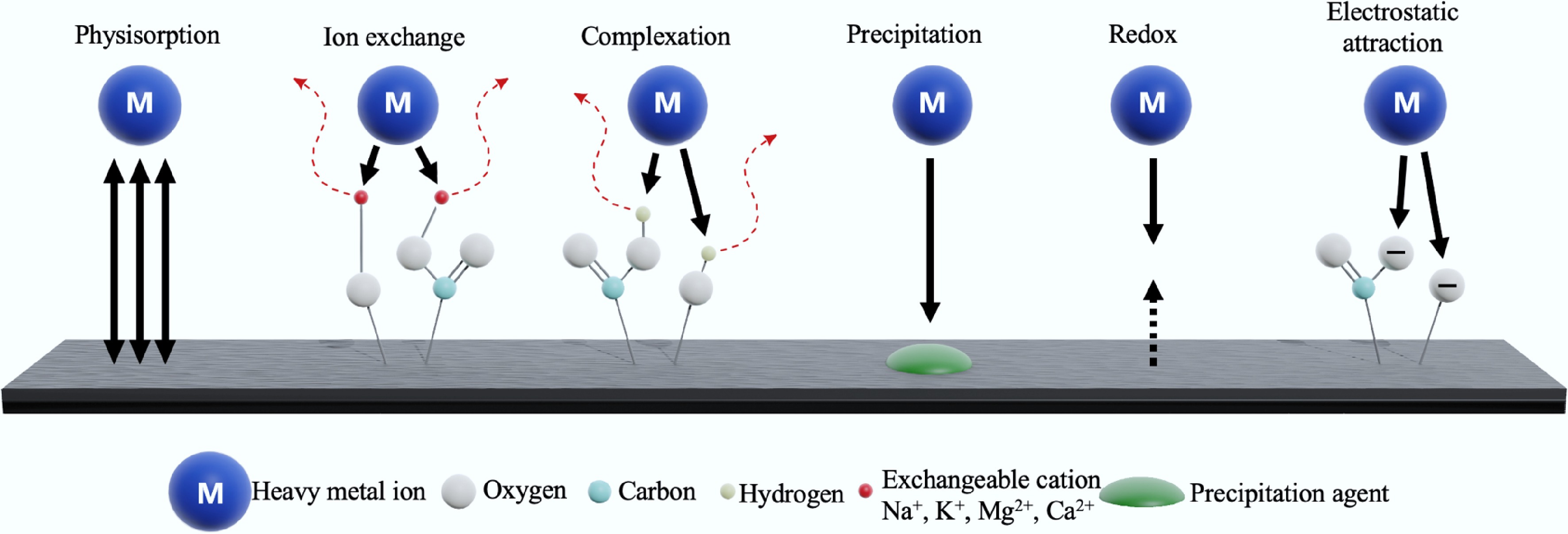
Figure 15.
Schematic diagram illustrating major metal ion removal mechanisms on carbon materials surfaces.
-
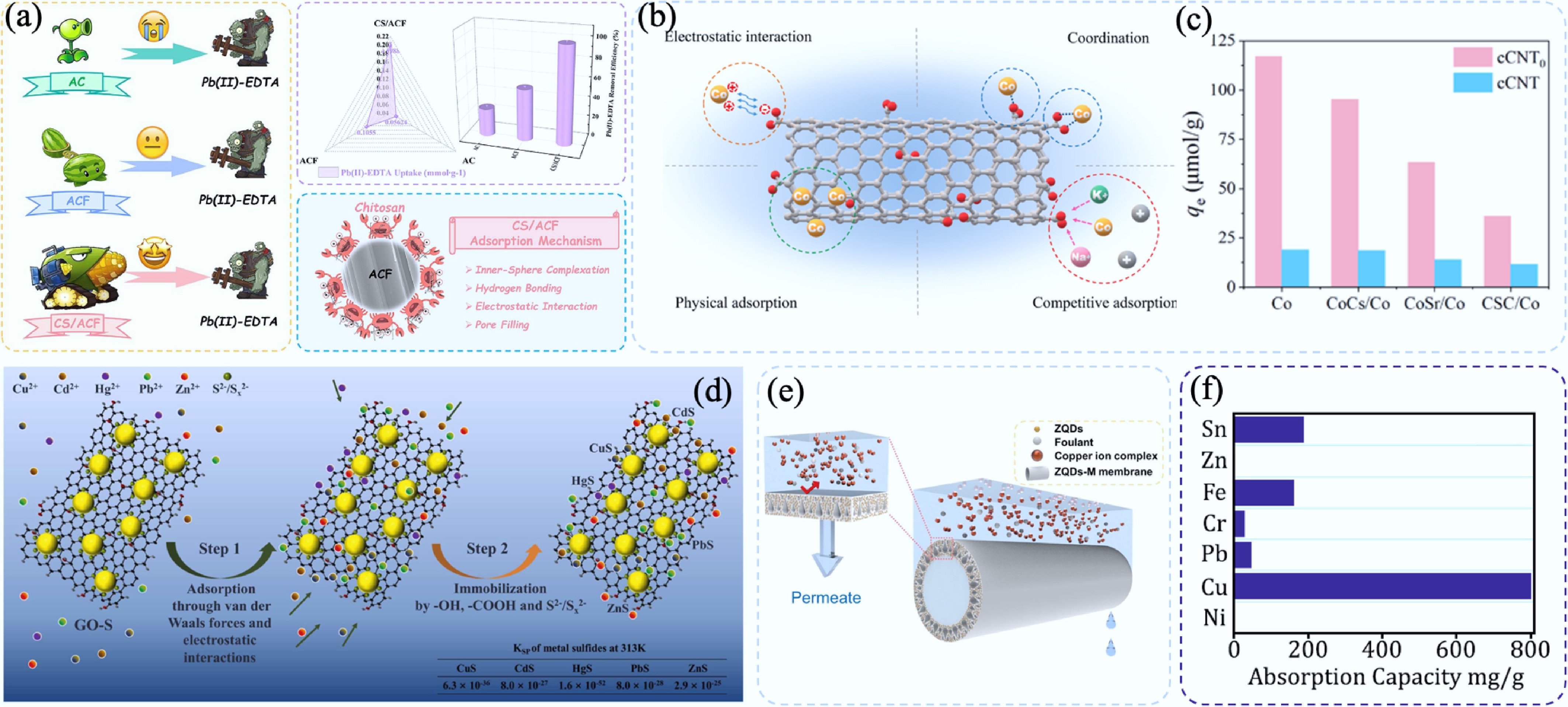
Figure 16.
(a) Schematic diagram of functionalized CS/ACF and its adsorption performance for Pb2+-EDTA[372]. (b) Schematic diagram showing the adsorption mechanism of cCNT and (c) adsorption capacity of Co2+ in simulated seawater[387]. (d) Schematic diagram of the mechanism of heavy metal ions adsorbed by GO-S[395]. (e) Schematic diagram of ZQDs-M removal Cu2+[401] and (f) adsorption capacities of CA for a variety of heavy ions[402].
-
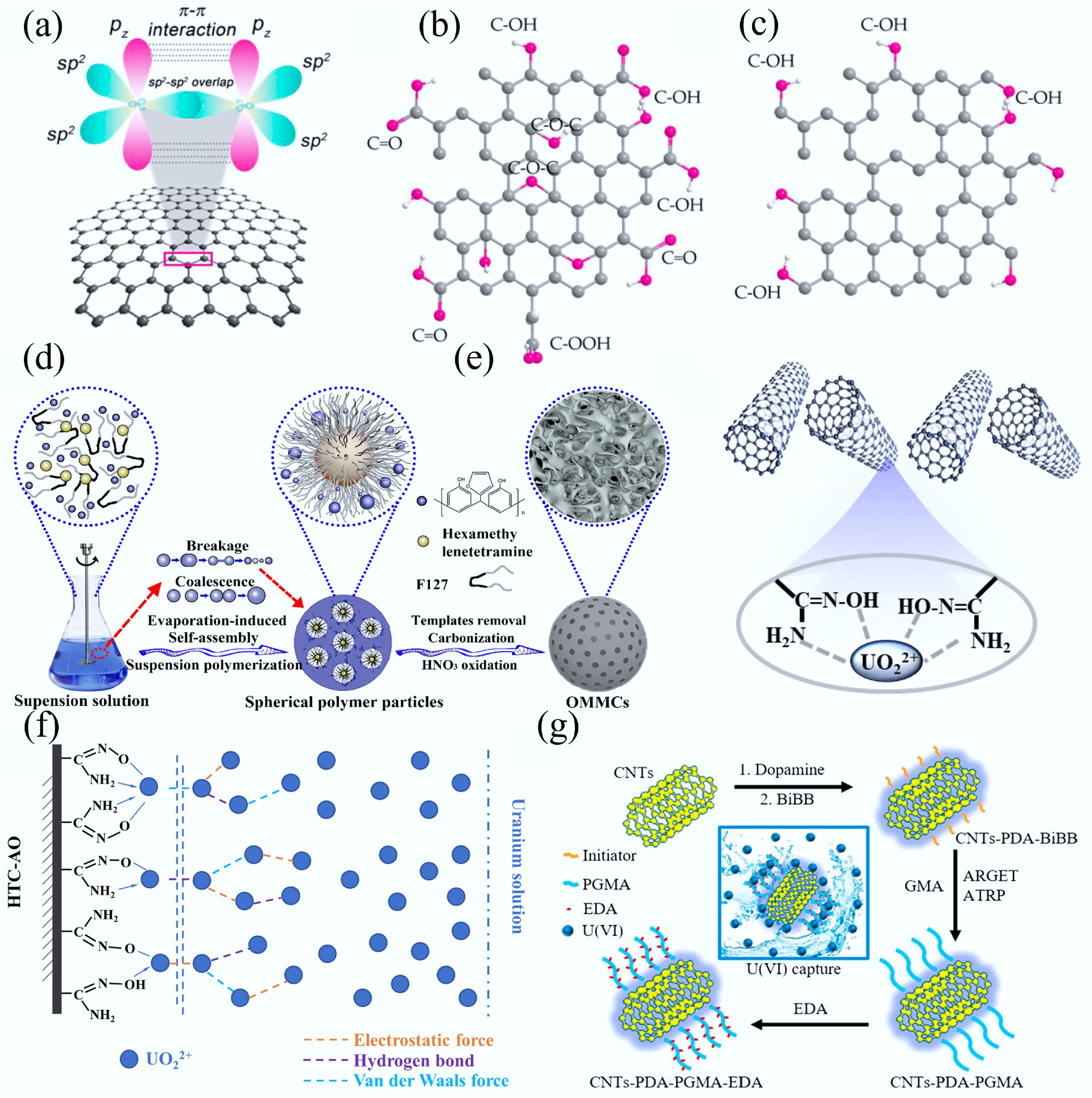
Figure 17.
Structural representations: (a) Pristine graphene. (b) GO. (c) Reduced GO[414]. (d) Schematic illustration of the synthesis of OMMCs[415]. (e) Probable sorption mechanism of U(VI) on AO-g-MWCNTs[416]. (f) The proposed monolayer and multilayer sorption modes for uranium sorption onto HTC-AO[417]. (g) Schematic diagram of the synthetic route of CNTs- polydopamine (PDA)-PGMA-EDA[418].
-
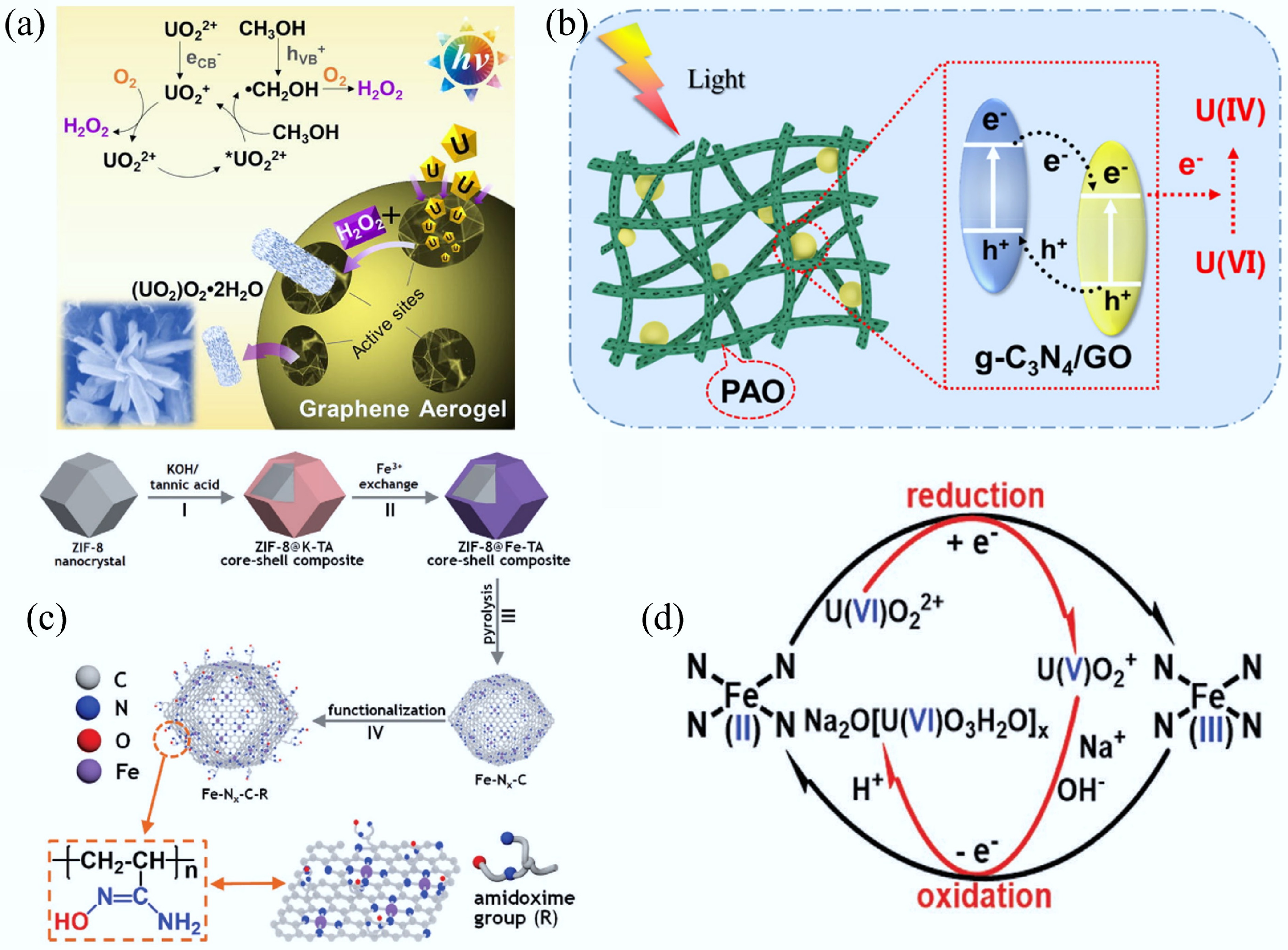
Figure 18.
(a) Illustration of graphene aerogel for the photocatalytic extraction of uranium under visible light irradiation and air atmosphere[456]. (b) Mechanism diagram of the photocatalytic extraction of U(VI)[457]. (c) Schematic illustration of the synthesis of Fe–Nx–C–R. (d) Schematic showing a plausible reaction mechanism for the Fe–Nx–C–R catalyzed extraction of uranium from seawater[35].
-
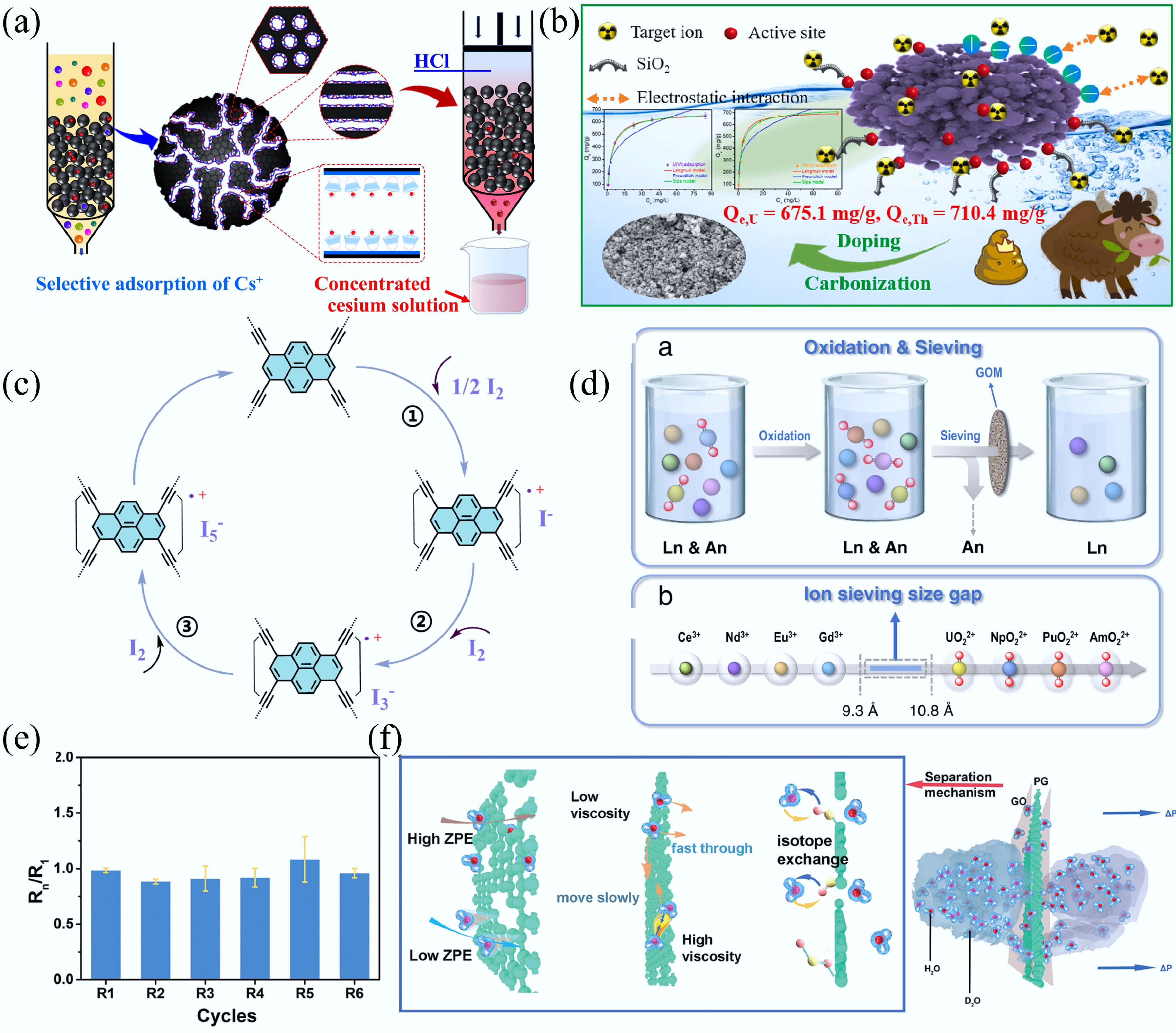
Figure 19.
(a) Mechanism for adsorption Cs(I) on C4BisC6/MMCs-P-5[470]. (b) Adsorption mechanism of U(VI) on TiO2@SiO2-CMBC[472]. (c) Mechanism of I2 uptake by PTEM[37]. (d) Scheme of actinides/lanthanides group separation and representative[473]. (e) Rejection rates with GO heterostructure membranes for the H2O/D2O. (f) Mechanism of GO/PG/GO separation of H2O/D2OM[474].
-
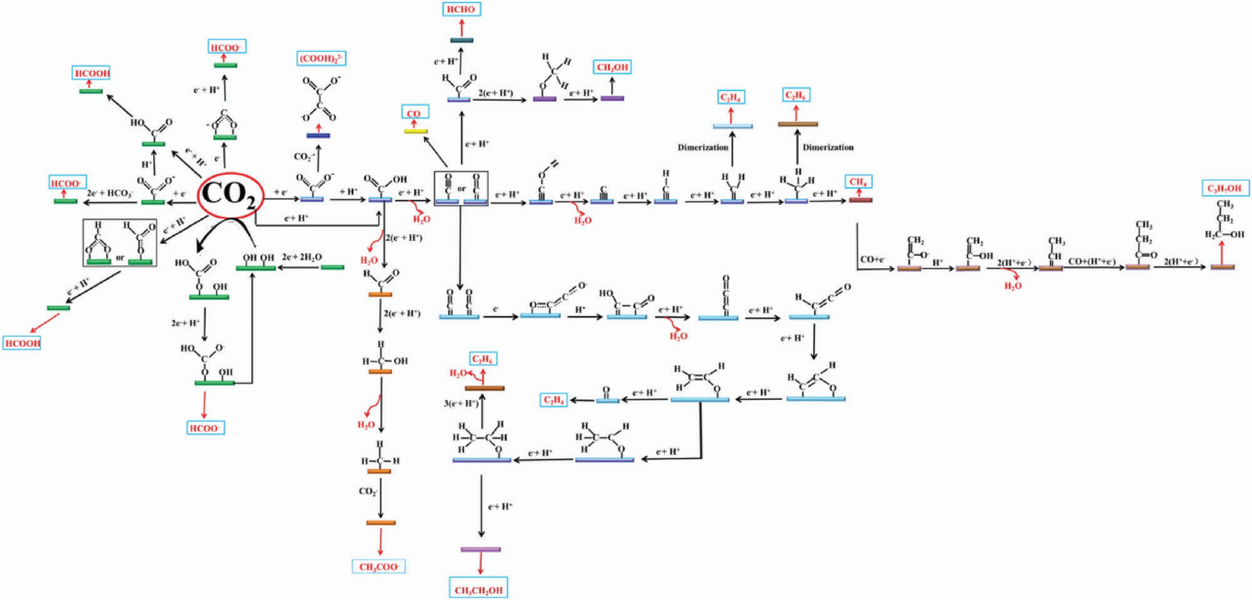
Figure 20.
The PCET pathway for CO2RR to carbon-based fuels[507].
-
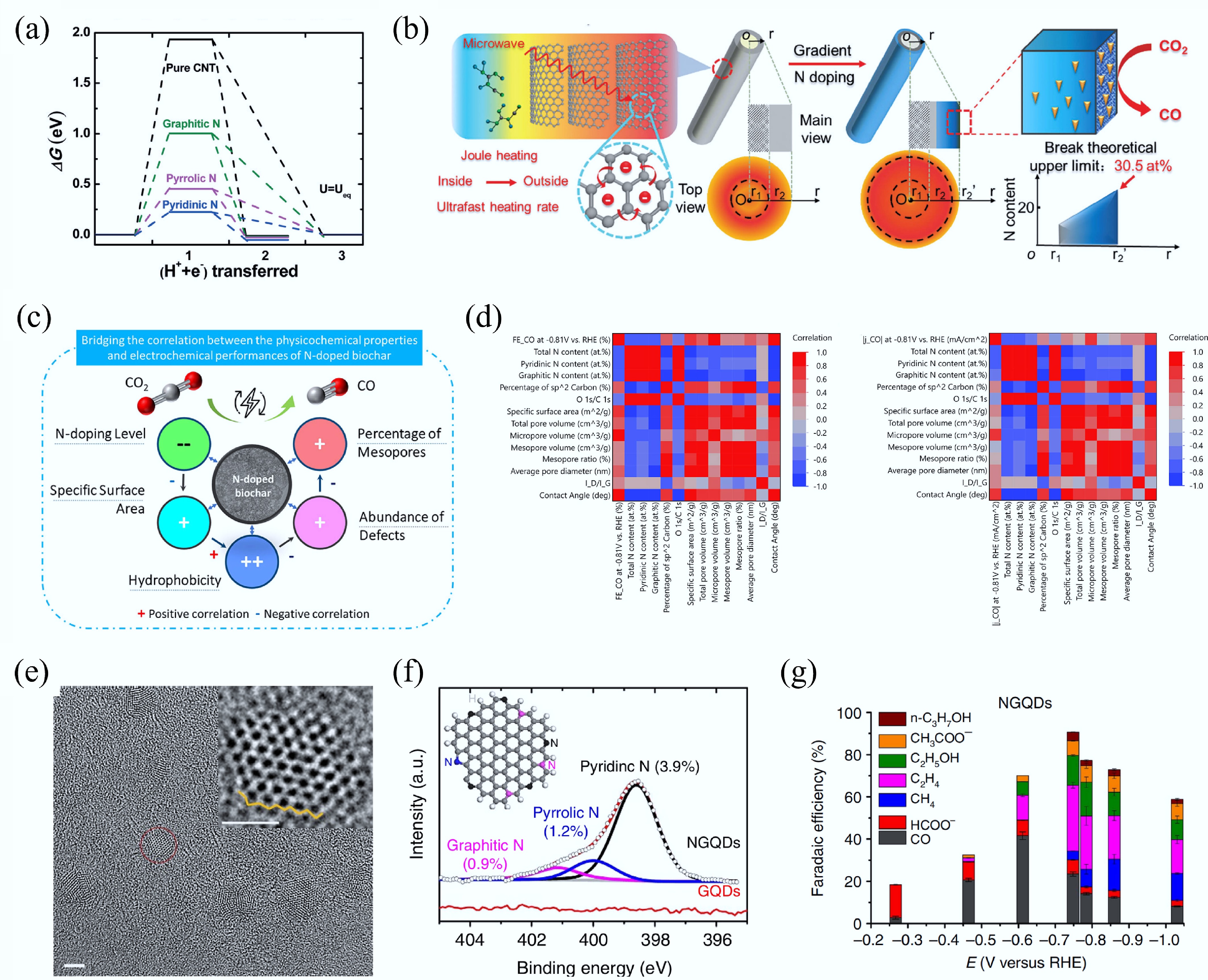
Figure 21.
(a) The Gibbs free energy diagram for CO2RR on different doping positions of N[12]. (b) Microwave irradiation synthesis of gradient nitrogen doping along the radial direction of CNT with ultrahigh N-content[511]. (c), (d) The influence of the structural parameters of N-doped biochar on CO2RR[514]. (e) The high-resolution transmission electron microscopy (HRTEM) image of NGQDs. (f) The N 1s XPS analysis of NGQDs. (g) The CO2RR over NGQDs[515].
-
-
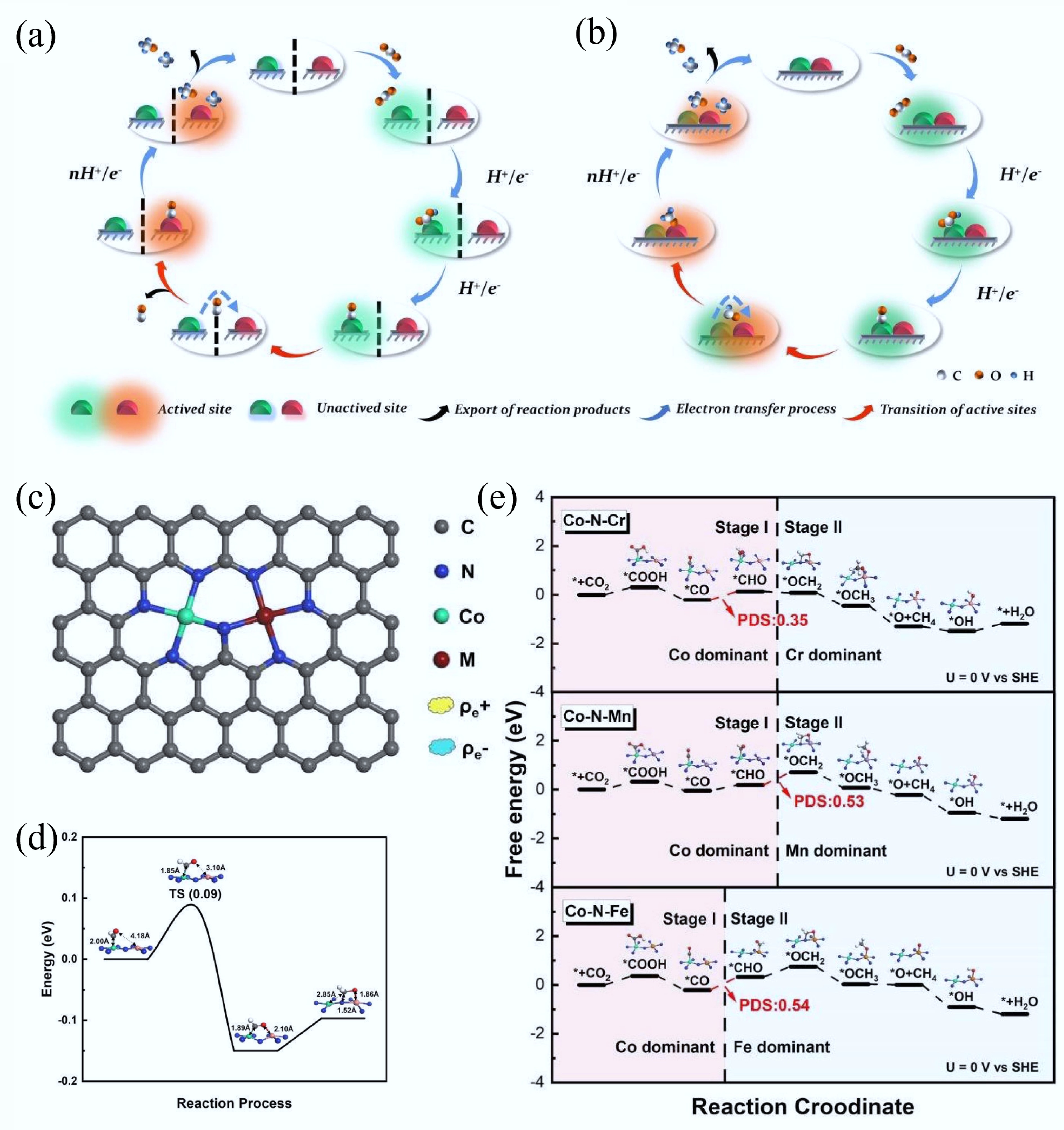
Figure 23.
(a), (b) Schematic diagram of the dynamic catalytic mechanism for the CO2RR on traditional tandem catalysts and inner tandem catalysts. (c) Model of Co–N–M inner tandem catalyst. (d) The activate barrier for the migration of adsorbed intermediates on Co–N–Cr inner tandem catalyst towards CO2RR. (e) The inner tandem reaction path for Co–N–M catalysts[38].
-
-
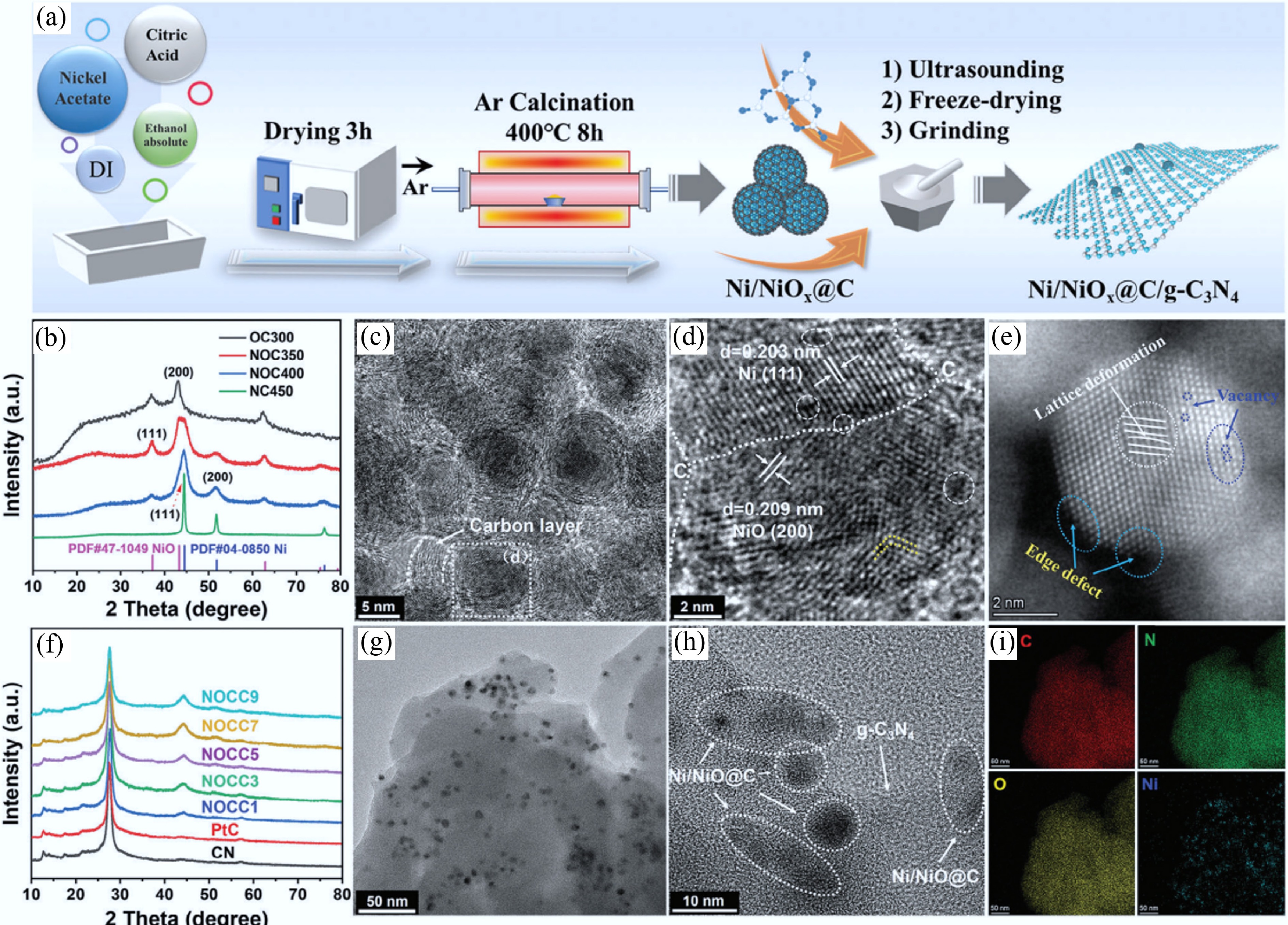
Figure 25.
(a) Schematic diagram of the preparation process of Ni/NiOx@C cocatalyst and Ni/NiOx@C/g-C3N4 photocatalyst. (b) XRD patterns of Ni/NiOx@C structures at different temperatures. (c), (d) Transmission electron microscope (TEM) images of Ni/NiOx@C samples. (e) Aberration-corrected high-angle annular dark-field scanning transmission electron microscopy of Ni/NiOx@C. (f) XRD patterns of Ni/NiOx@C/g-C3N4 with different loading amounts. (g), (h) TEM images, and (i) TEM/energy-dispersive spectroscopy mapping of NOCC5[544].
-
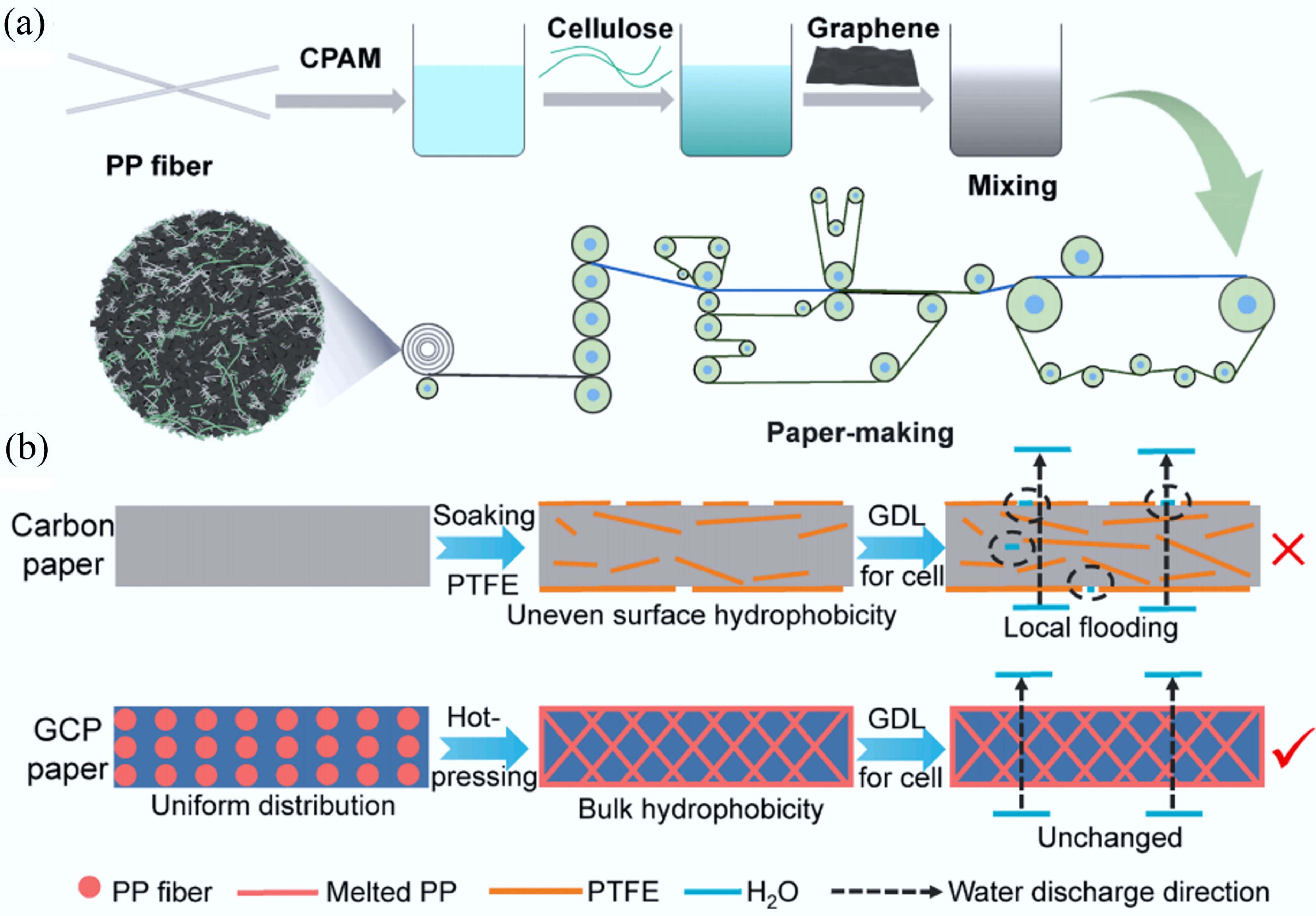
Figure 26.
(a) Preparation of GCP composite paper through wet papermaking process. (b) GDL based on GCP paper has uniform bulk hydrophobicity and better water management ability compared to traditional carbon paper GDL. Reprinted with permission from Tang et al.[549].
-
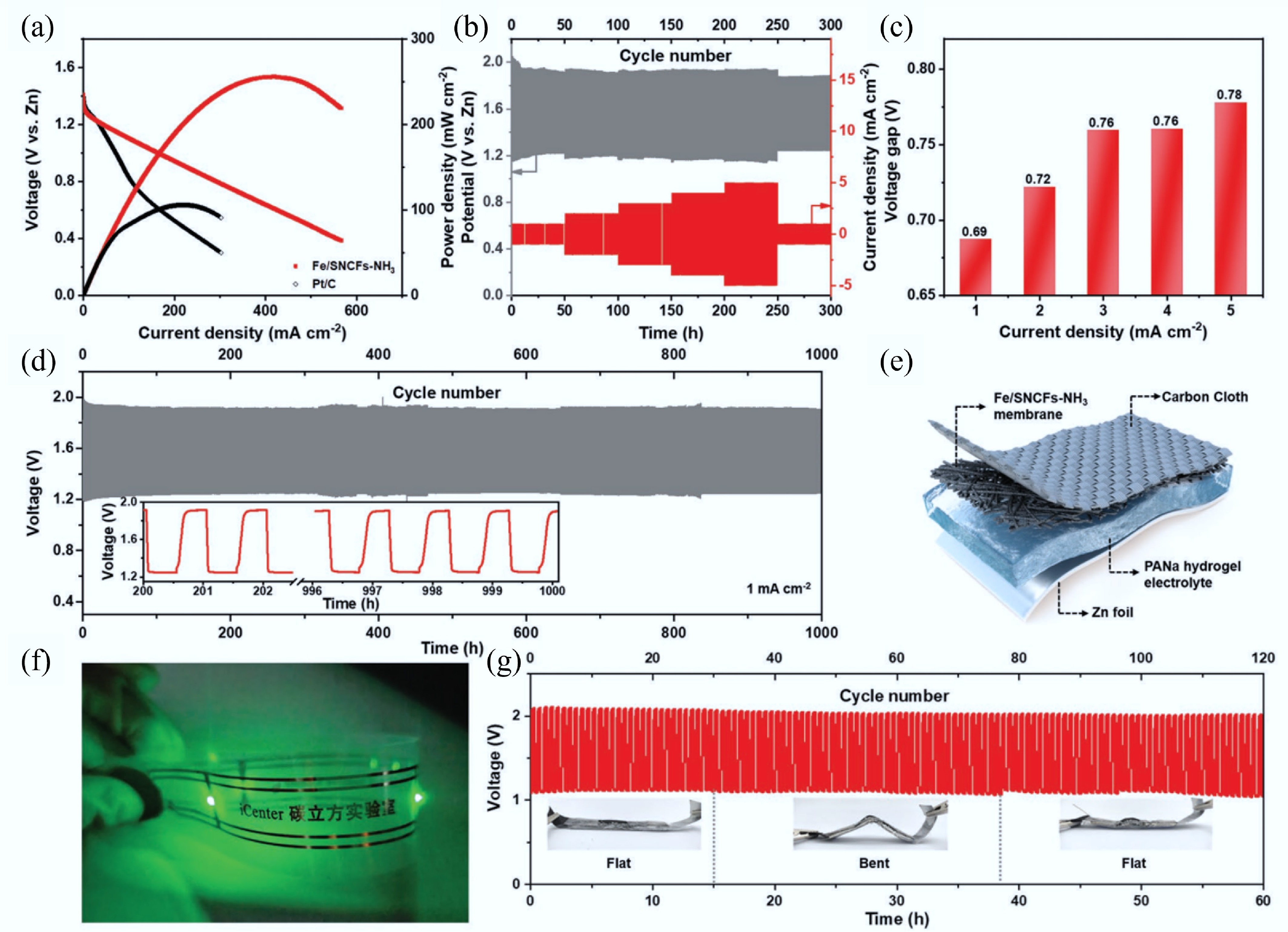
Figure 27.
Zn–air batteries (ZABs) performance of Fe/SNCFs-NH3 catalyst as an air cathode. (a) Discharge polarization curves and corresponding power densities of liquid-state ZABs. (b) Charge-discharge curves of the liquid-state ZAB at different current densities ranging from 1 to 5 mA/cm2. (c) Histogram of the voltage gaps at different current densities. (d) Long-term cycling stability at 1 mA/cm2 of the liquid-state ZAB, and inset is the enlarged charge and discharge curves. (e) Simplified schematic of the solid-state ZAB using a sodium polyacrylate (PANa)-KOH-Zn(CH3COO)2 hydrogel as the electrolyte. (f) Photograph of a wristband with a series of LED lamps lightened by two series-connected solid-state ZABs. (g) Stability of the solid-state ZAB at 1 mA/cm2, and inset are the photographs of the solid-state ZAB at various flat/bent/flat states[40].
-
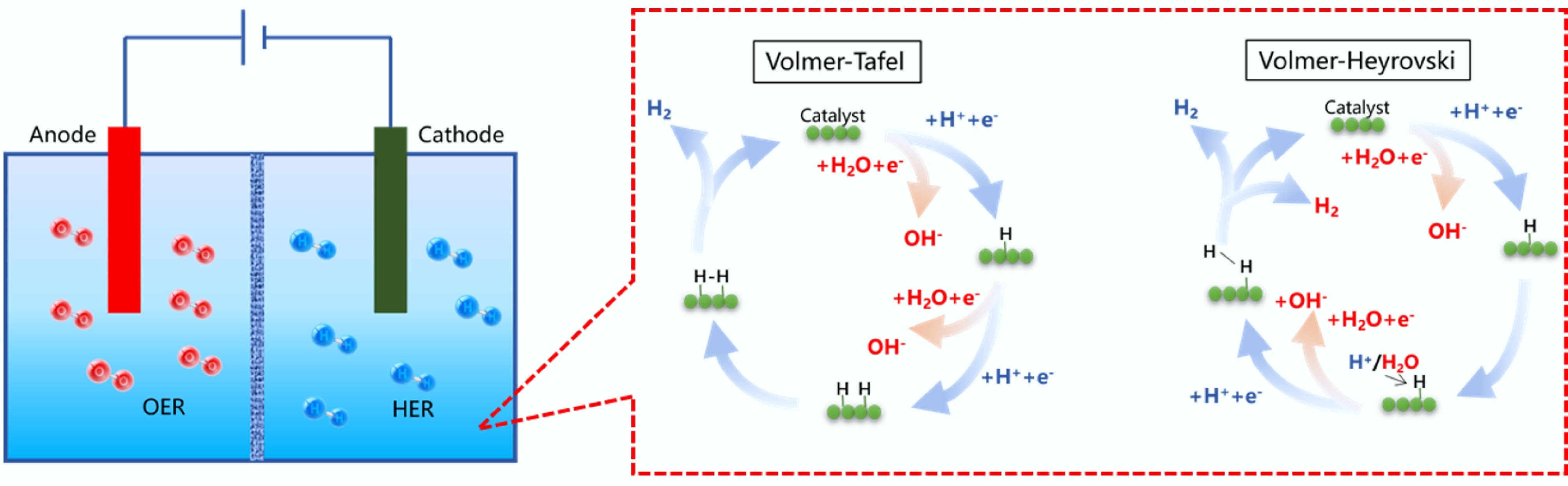
Figure 28.
The reaction steps of HER in acidic and alkaline electrolytes.
-
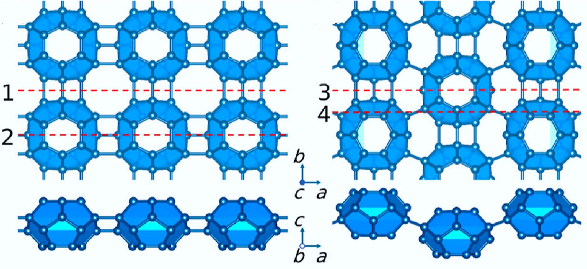
Figure 29.
Top and side view of the C24 monolayer crystal structure[560].
-
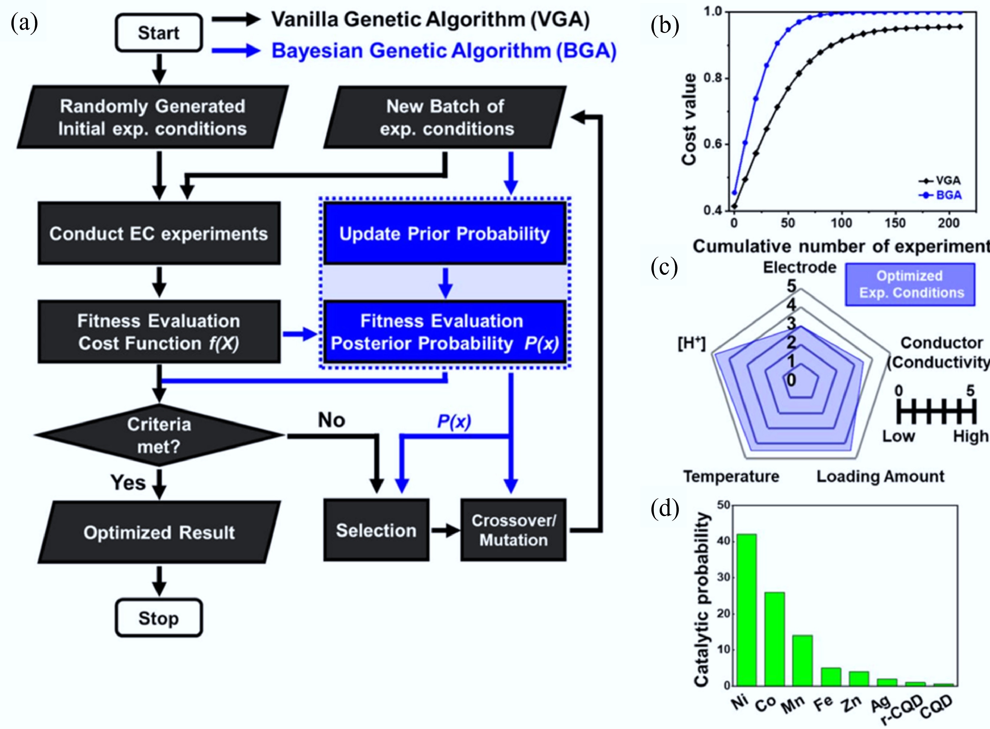
Figure 30.
(a) Flowchart of the proposed BGA and VGA. (b) Performance comparison between conventional GA optimization and BGA optimization for a generic convex-shaped cost function. (c) Score evaluation of important variables for electrochemical measurement. (d) Ranking of TM dopant in CQD toward catalytic performance[567].
-
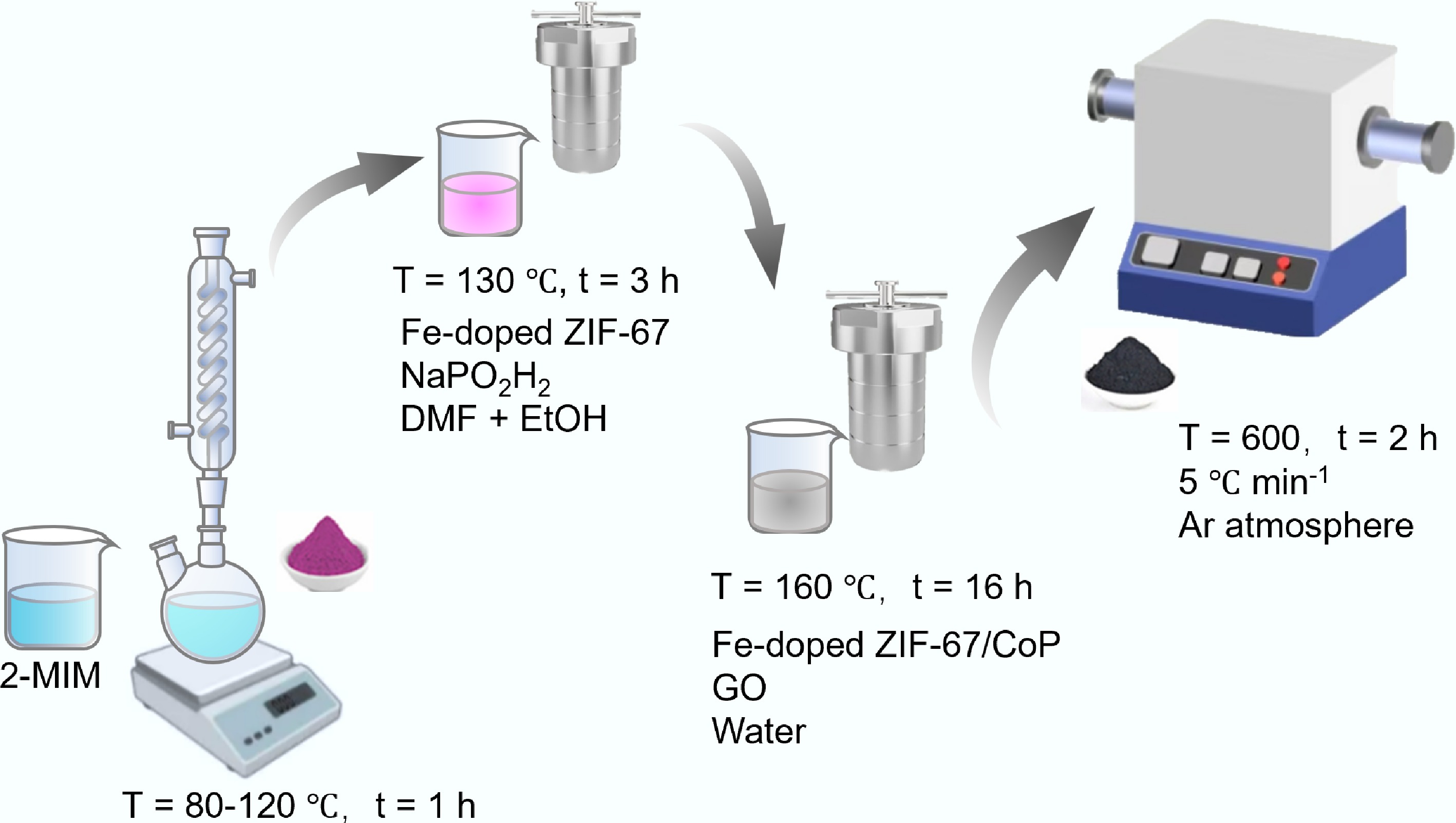
Figure 31.
Synthesis of Fe-CoP@NC/N-rGO hybrid composites derived from ZIF-67 MOFs.
-
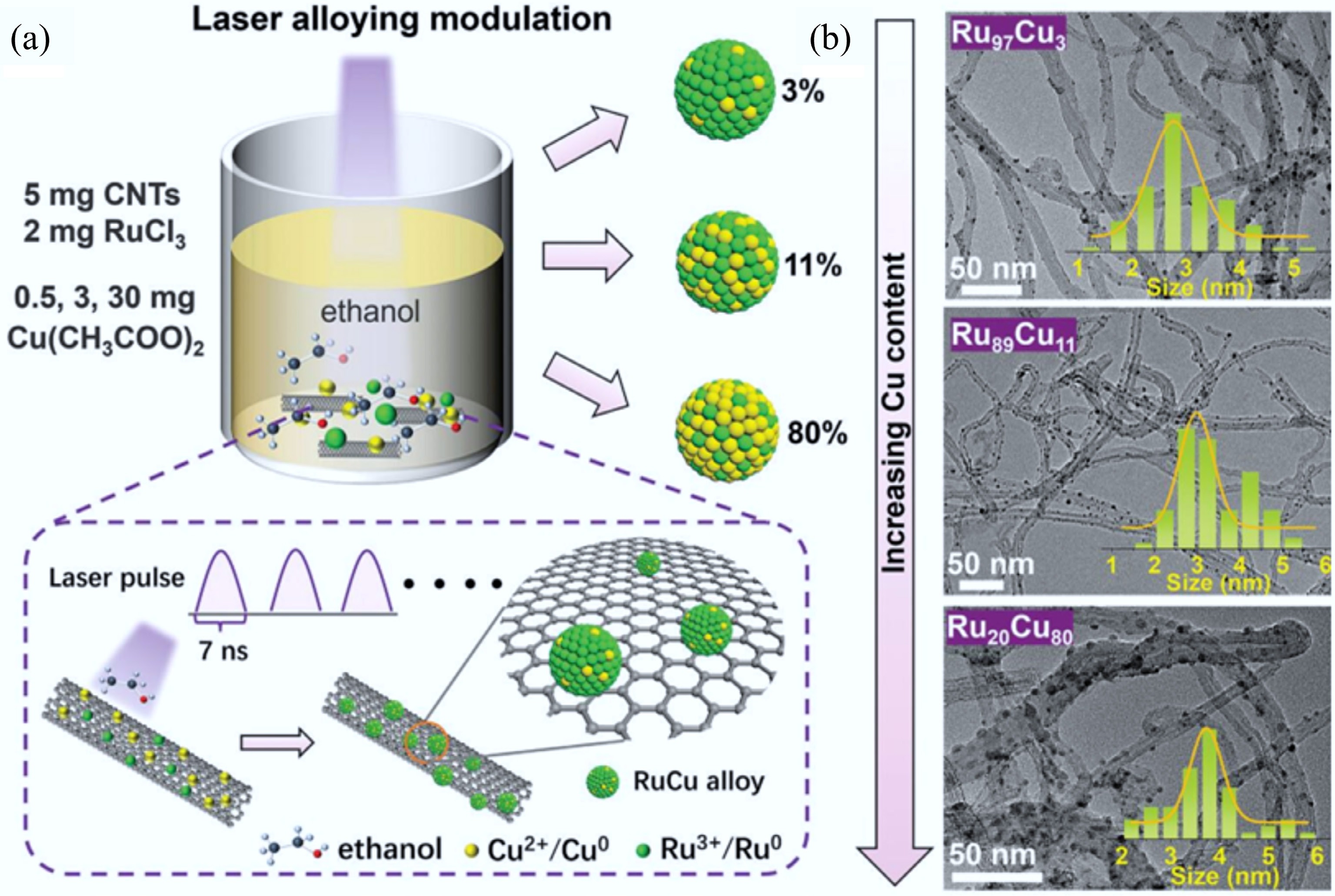
Figure 32.
(a) RuCu alloy composition modulation by LUCA. (b) TEM images of RuCu/CNTs and their size distributions[586].
-
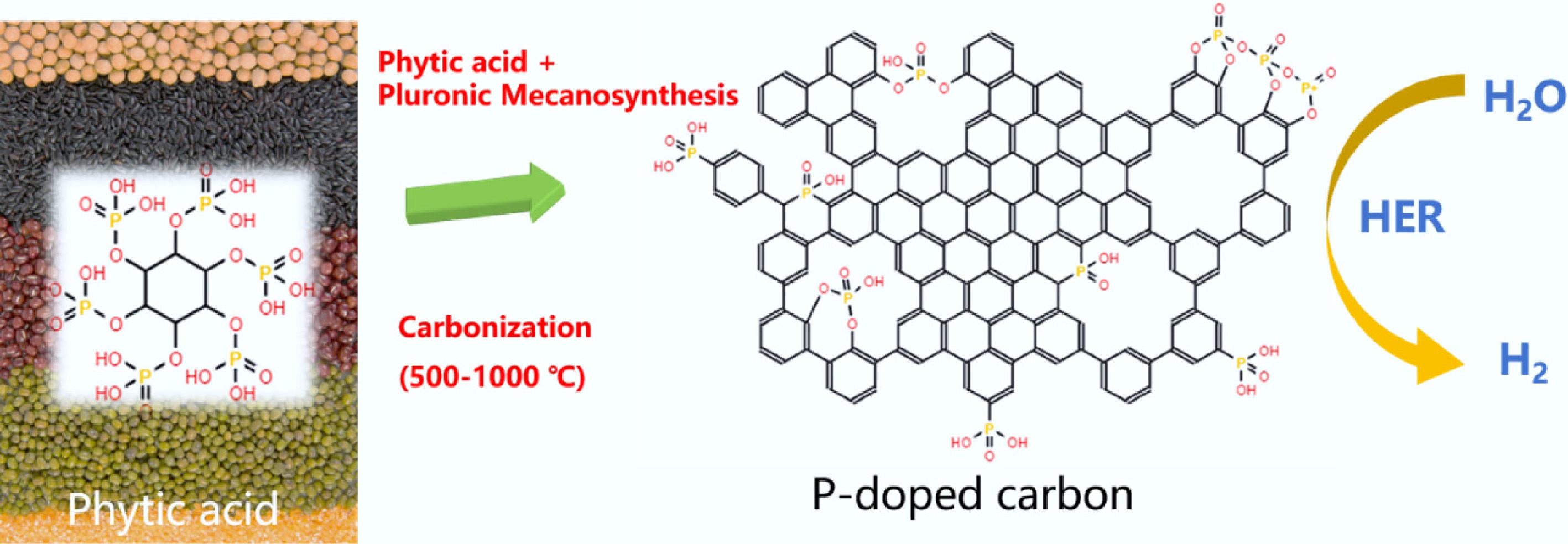
Figure 33.
Schematic of the synthesis process of P-doped carbons from phytic acid.
-
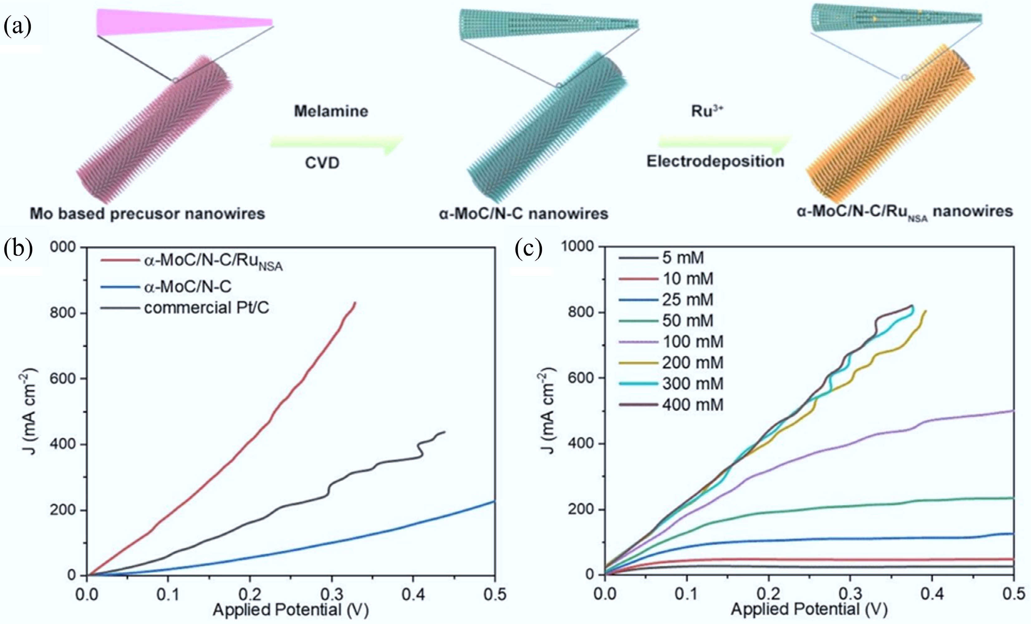
Figure 34.
(a) The schematic illustration of the formation of α-MoC/N−C/RuNSA. (b) Evaluation of the overall hydrazine splitting performance. (c) The overall hydrazine splitting in simulated alkaline sewage with different N2H4 concentration[596].
-
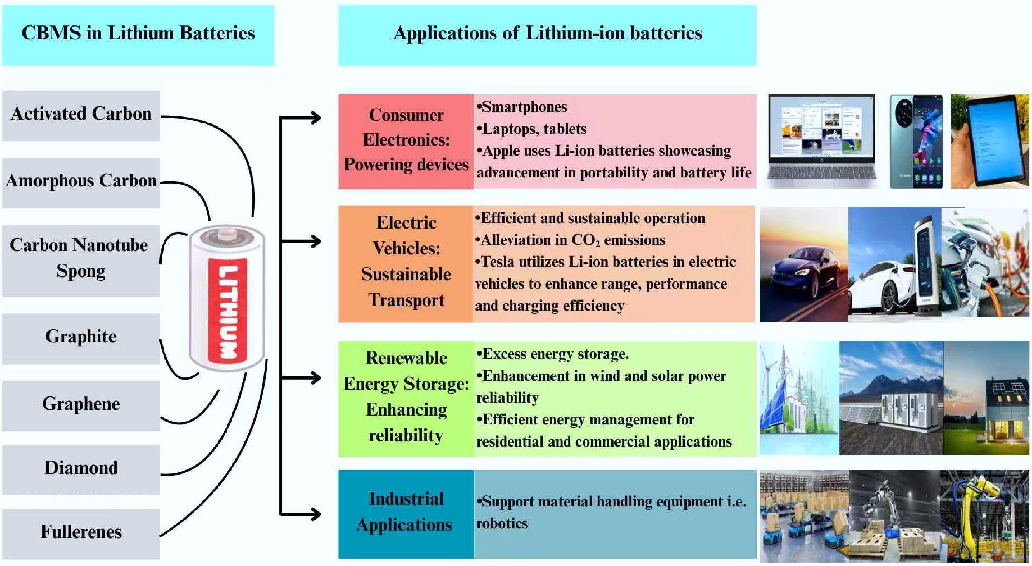
Figure 35.
Applicability of CMs in LIBs.
-
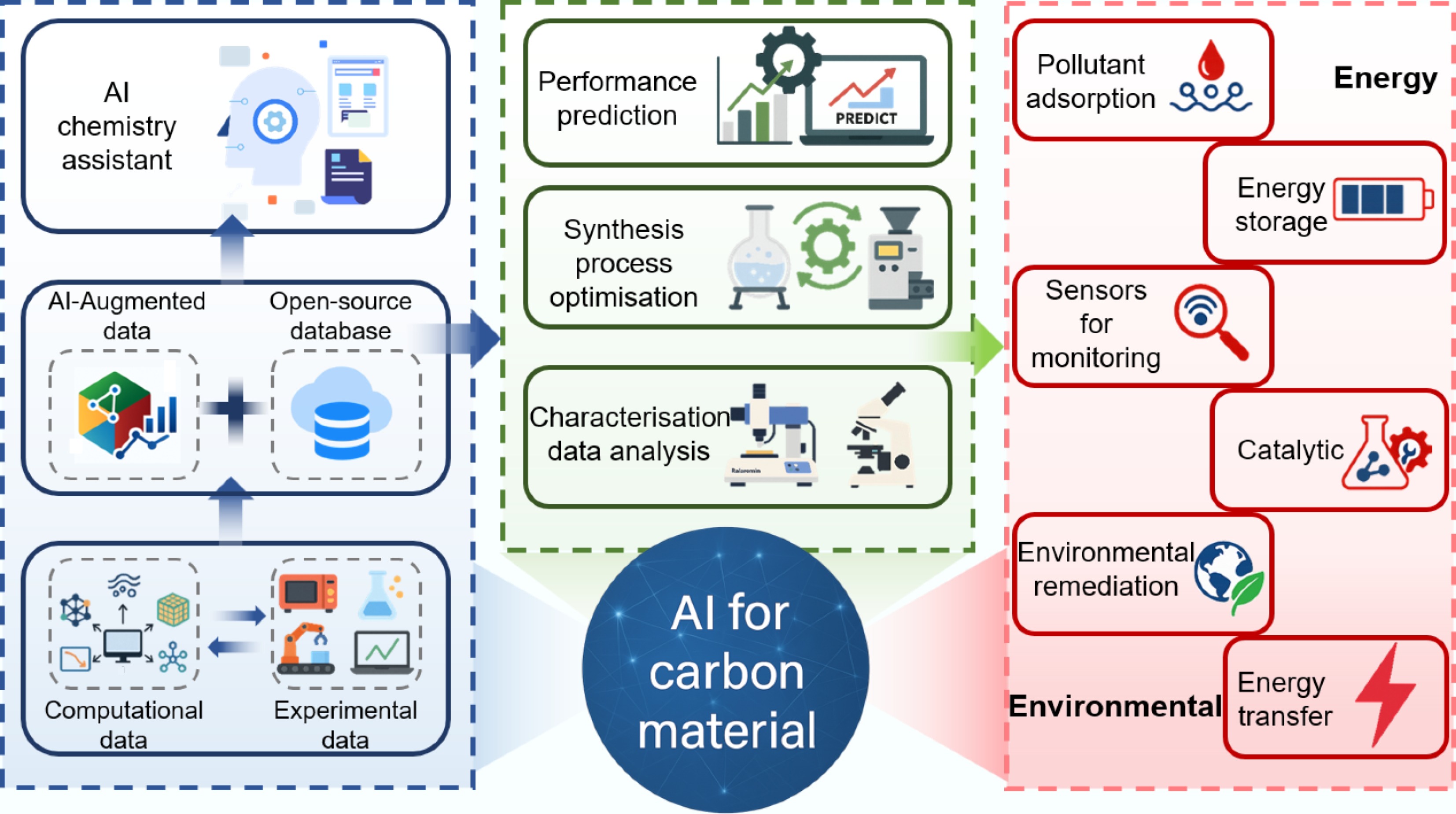
Figure 36.
Schematic overview of several insights into the development of AI approaches in CMs for various practical applications.
-
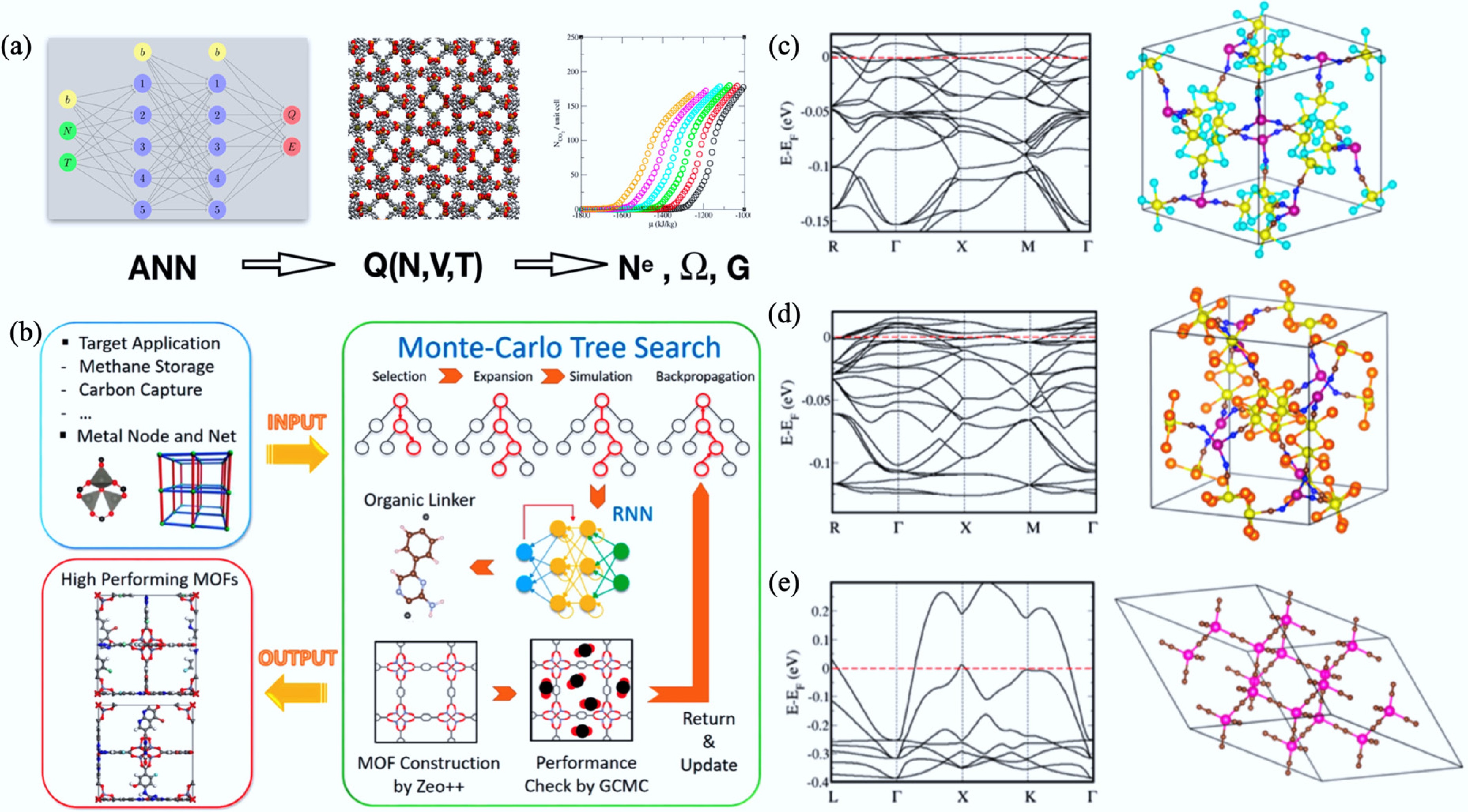
Figure 37.
(a) Schematic illustration of an ensemble learning framework integrating ANNs to predict the partition functions of adsorbed fluids in metal–organic and COFs[715]. (b) Representation of the Monte Carlo tree search and recurrent RNN framework for the inverse design of application-specific MOFs[713]. (c)–(e) Optimized crystal structures and calculated electronic band structures of three DFT-confirmed metallic MOFs—Mn9Re24C24S32N24, Mn9Re24C24Te32N24, and Mn9Re24C24Se32N24—highlighting their zero band gaps and potential electrical conductivity[711].
-
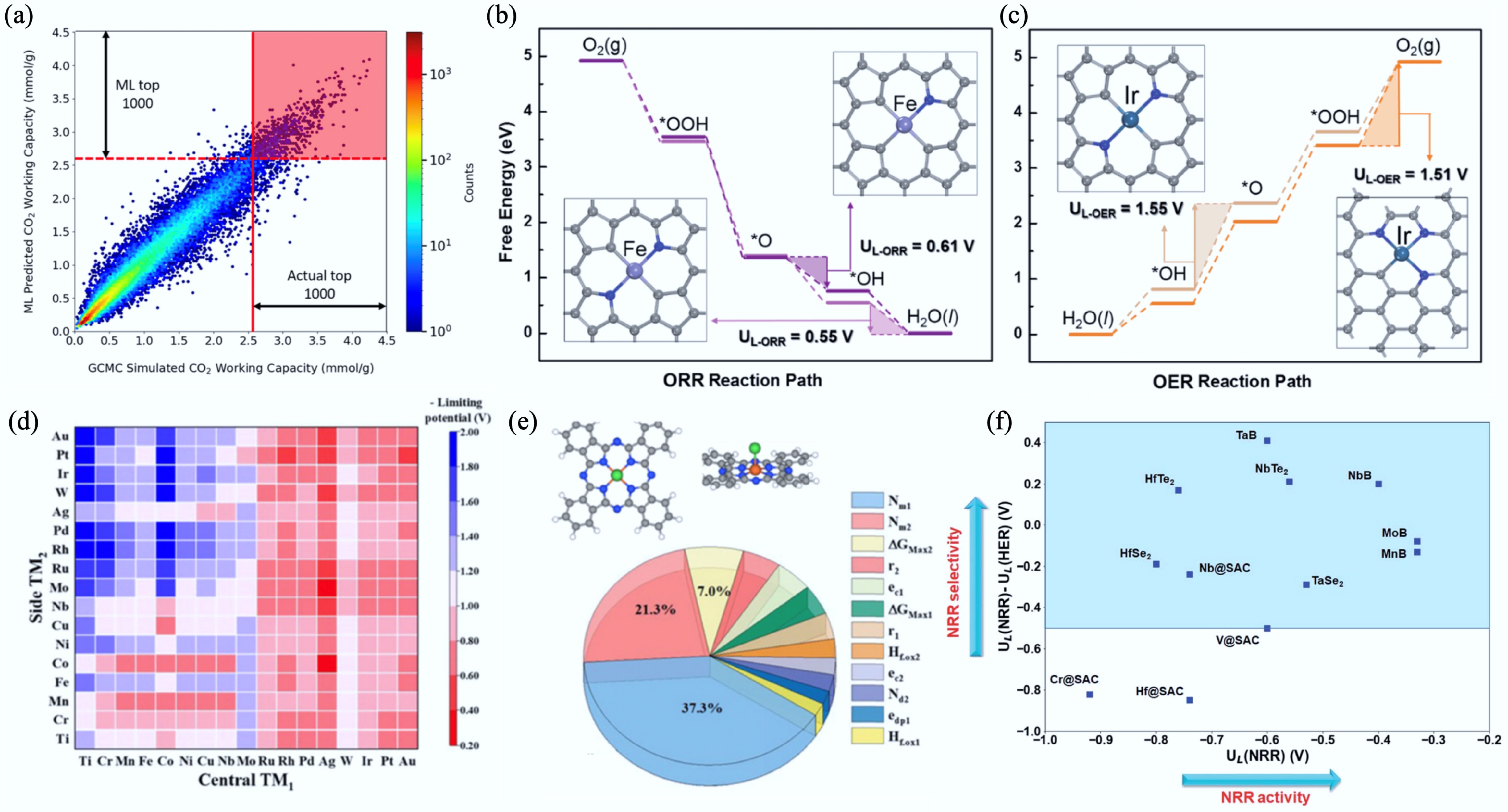
Figure 38.
(a) Heat map showing the correlation between ML-predicted CO2 working capacity and Grand Canonical Monte Carlo-simulated CO2 working capacity for MOFs[724]. (b) Heat map of ML-predicted theoretical limiting potentials for Pc DACs; the redder, the better the catalytic activity for the CO2RR. (c) Feature importance analysis highlighting the top 12 descriptors (contribution 41.5%)[726]. (d), (e) Free-energy diagrams and geometries of prominent M@NₓCᵧ SACs for the ORR and OER, at zero electrode potential. The rate-determining steps are highlighted by shades, and the blue and gray balls represent nitrogen and carbon atoms, respectively[727]. (f) Visual comparison of limiting potentials for the NRR and the HER for various SACs and related materials[728].
-
Methods Year developed Advantages Limitations Products Refs. Carbonization (pyrolysis) 1980s Low cost, scalable, tunable porosity via precursors (e.g., biomass, polymers) High energy input (> 600 °C), Limited crystallinity (ID/IG > 1.5), amorphous morphology AC, biochar, carbon NPs, carbon foam [42,729] Hard templating 1990s Precise pore size control (2–50 nm), ordered architectures, high surface area Toxic template removal (HF/NaOH), low yield, high cost Ordered mesoporous carbon, CNTs, 3D carbon frameworks, CAs [489,730] Soft templating 1990s Template-free, self-assembly, tunable mesopores (2–10 nm) Poor thermal stability (< 400 °C), surfactant residue contamination Mesoporous carbon spheres, CNFs [731,732] CVD 1960s
(modern: 2004)High crystallinity (ID/IG < 0.1), atomic-level thickness control High cost, slow growth rate, substrate limitations Graphene, CNTs, carbon fibers (CFs), fullerenes, graphdiyne [53,733] Mechanical exfoliation 2004 Simple (e.g., Scotch tape), minimal chemical defects, preserves intrinsic properties Low yield (< 5%), non-uniform flake sizes, labor-intensive Graphene nanosheets, few-layer graphdiyne [734] Chemical exfoliation 2008 High yield, solution-processable, scalable Defect generation (ID/IG >1.0), requires harsh oxidants (H2SO4/KMnO4), residual functional groups Graphene oxide, CQDs [735] Electrochemical exfoliation 2012 Mild conditions (room temp), tunable surface groups, high purity (> 95%) Limited to conductive precursors, low throughput, solvent dependency Few-layer graphene, fluorinated CNTs [62,736] Chemical etching 2010 Defect engineering (edge sites), hierarchical porosity, enhanced surface reactivity Over-etching risks, corrosive reagents (HNO3/KOH) Holey graphene, porous CNFs [63,65] Physical etching 2015 No chemical waste, plasma/ion beam precision (nm-scale), high reproducibility High equipment cost, slow processing, limited to thin films Patterned graphene, nanoperforated carbon membranes [66,737] HTC 2001 Eco-friendly (aqueous, < 200 °C), spherical morphology control Low graphitization (ID/IG > 1.5), limited surface area (< 500 m²/g) Carbon microspheres, hydrochar from biomass, CQDs [68,69] CO2 utilization 2015 Carbon-negative process, converts waste CO2 Energy-intensive (600–1,000 °C), low efficiency (< 30% conversion) CNTs, graphene, fullerenes, PC [70] FJH 2019 Ultrafast (< 1 s), energy-efficient (~0.1 kWh/kg), upcycles waste precursors Limited to conductive precursors, non-uniform heating in bulk samples Turbostratic graphene, 3D PC, CQDs [64] Table 1.
Comparison of various synthesis strategies for CMs
-
Carbon material Absorption range (nm) Emission range (nm) Quantum yield (QY) Bandgap (eV) Graphene UV - NIR (200–2,500) 400–800 1%–74% ~ 0–3.6 eV Biochar UV - NIR (250–800) N/A N/A 0.1–1.0 CDs UV-NIR (200–1,800) 450–800 1%–85% 1.7–3.3 CNTs UV - NIR (200–2,500) 900–1,600 N/A ~ 0.1–0.5 Carbon fibers UV - NIR (250–2,500) N/A N/A ~ 0–0.01 AC UV - NIR (250–2,500) N/A N/A N/A Table 2.
Summary of photophysical properties of carbon-based materials
-
Heavy metal Major environmental sources Toxic effects on human health Ref. Pb Battery manufacturing, paint, contaminated soil, old plumbing Neurotoxicity, cognitive impairment in children, kidney damage, hypertension [738] Hg Coal combustion, gold mining, seafood (methylmercury) Neurotoxicity, tremors, vision/hearing loss, developmental defects in fetus [739,740] Cd Industrial emissions, phosphate fertilizers, smoking, mining Renal dysfunction, bone demineralization (Itai-itai disease), cancer [741] As Groundwater (natural/geogenic), mining, pesticides The most poisonous heavy metals, skin lesions, cancer (lung, bladder, skin), cardiovascular diseases [742] Cr Electroplating, leather tanning, pigments, steel manufacturing Carcinogenic, respiratory tract irritation, skin ulcers [743] Ni Stainless steel production, electroplating, combustion Dermatitis, lung fibrosis, carcinogenic potential (inhalation) [744] Cu Mining, plumbing, industrial waste, pesticides Gastrointestinal distress, liver/kidney damage at high doses [745] Zn Galvanized metal, industrial discharges, fertilizers Nausea, vomiting, immune system suppression (at excessive levels) [746] Mn Welding fumes, industrial emissions, contaminated water Neurological disorders resembling Parkinson's disease [747] Table 3.
Heavy metals and their sources, toxic effects
-
Carbon materials Dosage
(g/L)Heavy metals Initial concentration
(mg/L)pH Temperature* (°C) Time
(min)Adsorption capacity
(mg/g)Removal efficiency (%) Reusability Ref. ACs BAC 0.1525 Pb2+ 0.2 − 25 120 1.21 95% Reuse of spent AC [366] 0.1032 Cd2+ 0.50 86% RAC − Hg2+ − 5.5 25 360 109.05 ~100% ~100% by MWH after five cycles [382] CS/ACF 1 Pb2+−EDTA 0.2 mM 7 25 30 − 99.40% Stable after 10 cycles of regeneration [372] APS oxidized ACF 2 Pb2+ 4.5−5.0 25 120 559 − − [377] Thiol functionalized activated CF Pb2+ 100 5.5 25 120 700.77 − Adsorption capacity remain 150 mg/g after five cycles. [378] Sulfur-modified AC 5 Cd2+ 1,000 6.0 25 240 139 27.8 − [376] CNTs e-MWCNTs 100 As(V) 0.047-10.2 3 35 45 12.18 − − [381] MWCNTs/MnO2 0.2 As(V) 20 5.5 25 60 − 95% Can be regenerated [748] cCNTs 0.2 Co2+ 10 5.7 30 < 60 25.1 − − [387] CNTs 0.5 Pb2+ 2-14 7 25 6 h 17.5 87.8 − [379] CNT-S 1 Hg2+ 10 6 25 90 151.5 Around 13% and 17% dropped in second and third cycle, separately [740] GOs GO/UiO-66-NDC 2.5 Cr(VI) 10 mM 3 25 150 157.23 96.4% Dropped to 71.23% after six cycles [391] GO 0.1 Cu2+ − 5 25 120 294 − − [394] Zn2+ 345 Cd2+ 530 Pb2+ 1,119 GO-AG 0.03 Cd2+ − 3-4 25 12 h 1,792.6 − − [390] DGSP 1 Cu2+ 20 5 30 240 208 Remained at 71.54% of the initial removal efficiency after five cycles [393] GO-S 0.05 Cu2+ 150 5 25 60 678 − Remain at 83% of the initial removal efficiency after five cycles [395] Cd2+ 646 Hg2+ 565 Pb2+ 683 Zn2+ 490 CDs FH-5 − Cr(VI) − − − < 120 534.4 − − [400] Ba2+ 271.9 Pb2+ 789.6 Cu2+ 98.2 ZQDs-M − Cu2+−SDDC 4 ppm Cu2+
10 ppm SDDC10 25 − − 95.4%
(pure water flux of 6,227.4 L/[m2·h1·bar1])Remain 73.4% flux recovery ratio after three cycles [401] CD/HPMC/SiO2 1 Pb2+ 1,000 6 15 190 s 258.3 − Remain 90% for Pb2+ after three cycles, and for Co2+ after four cycles [399] Co2+ 5 20 300 s 168.1 CAs MCA 0.4 Cd2+ 60 mg/L 7 20 30 143.88 − Remain 93% of the initial removal efficiency after five cycles [403] Carbon aerogels 0.4 Cu2+ 400 25 12 h 801 − No obvious change after five cycles [402] CCA − Cu2+ − 7 25 10 55.24 − Remain 96% of the initial removal efficiency after five cycles [404] CA 1.6 Pb2+ − 4.5 − − 34.72 − − [749] Table 4.
Removal of heavy metals onto carbon adsorbents
-
Catalyst Main product FE (%) Current density (mA/cm2) Ref. N, P co-doped CAs CO 99.1 143.6 (partial for CO) [512] O-doped C2N CO 94.8 2.75 (partial for CO) [513] Co-S1N3 single-atom CO 98 200 [523] IPCF@CS CO 99.5 550 [521] Ni-N-C with high nanocurvature CO > 99% > 400 (partial for CO) [524] NiPc on multi-wall CNT CO 99.5 300 [530] NGQDs C2H4 and C2H5OH 45 46 (partial for C2H4); 21 (partial for C2H5OH) [515] B, N co-doped nanodiamond C2H5OH 93.2 Not mentioned [518] Cu2N6 C2H4 52 180 [525] Curved CoPc on single-wall CNT CH3OH > 60 > 90 (partial for CH3OH) [531] Nitrogen-doped nanodiamonds/Cu interface C2 oxygenates 63 Not mentioned [533] Composite Cu and F-doped carbon Multicarbon products 82.5 400 [534] Table 5.
A comparison of FE and partial current density of SCMs for CO2RR
-
Table 6.
Comparative OER activity with metal free carbon based materials and TDA-Trz-POP
-
CMs Applications Purpose Ref. Country (year) BC-MWCNT composite Potential antiviral agents, wound healing Anti-oxidant function, healing of diabetic wound,s and controlled cytokines expression, [751] Pakistan, 2022 BCDs Bio-imaging, biosensor, energy storage Used commonly, Food safety, aureus detection, mode sensing, and radiometric fluorescence [657] China, 2023 CNTs It plays crucial role in drug delivery system Stem cell culture, assisting drug release into cells, biosensing, delivery of doxorubicin to cancer cells [654] Turkey, 2022 CDs with red emission Cancer therapy, bioimaging, biosensing Successful detection of bio thiols, rapid cell internalization [752] India, 2021 MWCNTs Biomedical imaging, tissue engineering, drug delivery system Enhanced bioavailability, targeting tumor site drug delivery, cytotoxicity, HeLa cells [753] Brazil, 2023 Gc-NPs Biosensing, tissue engineering, bioimaging High protein adsorption capacity, imaging of sentinel lymph nodes [97] USA, 2013 Fullerene/Buckyball Photo-sensitizers, wound healing, anti-oxidant, Most commonly used in cancer especially breast cancer [754] China, 2019 GTCEnc Tissue engineering, anti-cancer, wound healing Anticarcinogen, and antimicrobial activity, mostly progressive against COLO205 cell lines [755] Saudi Arabia, 2023 NDs Diagnostics, and wound healer tool Tissue engineering, and neural regeneration and [664] Iran, 2023 Table 7.
Application of CMs in biomedical sciences
-
CMs Promising characteristics Applications Ref. Country Applications of CMs in food the industry F-C60 Biological sensor, antioxidants Food quality, food safety, increase caloric value [756] Germany C-Ar Verstyle stability, host of ingredients, culture media It increases shelf life, and also used in food packing [757,758] Italy BC It is highly porous, with a high surface area. Antimicrobial Sustainable food production, waste management, food preservation [688] Korea AC Surface chemistry, adsorption potential, It plays a key role in decolorization, deodorization, and purification [759] India CDs It acts as a biosensor as well as a chemical sensor Detection of food additives, quality, food safety [760] Pakistan CNTs Antibody, antimicrobial properties, biosensing, immobilization, Ethylene production, food ripening, food packaging [761] Bangladesh G Bio and chemical sensor, antimicrobial properties Food safety and preservation, packaging and quality control [762] Pakistan CNFs It has antimicrobial and antioxidant properties Food packaging, quality control, and preservation of food [763] Hungary Applications of CMs in agriculture BC Carbon-rich material, cation exchange capacity, porous, high surface area Reduce soil acidity, high porosity, sequester carbon, improve soil health [686] Nepal F-C60 Free radical binding, resistance to radiation Antioxidant and Nrf2 activation, plant protection, potential for pest control [764] Thailand CNFs Graphene layer, cylindrical structure Plant protection, nutrients, nutrient delivery, carriers for pesticides [763] Hungary C-Ar Low density and porosity, high surface area Biopesticides and biofertilizers, soil amendment, nutrient delivery [687] Korea AC Surface chemistry, porous, high surface area, adsorption potential Control odors, filter water, nutrient availability, improve soil [765] Malaysia CDs Antioxidant and antimicrobial Stress resistance, accelerating plant growth [312,596] China CNTs Unique structural, special electronic, and mechanical properties Plant growth regulation, gene delivery, seed germination [766,767] Pakistan, India G Single layer of carbon atoms, high binding energy Improving soil health, antifungal, enhancing plant growth, antibacterial agents [232] United States Table 8.
Application of CMs in agriculture and the food industry
-
Model Application Advantages Disadvantages Ref. K-means clustering Structural clustering, feature selection Easy to implement; fast training; scalable to large datasets. Requires specifying the number of clusters (K); may not capture complex, non-linear feature relationships. [707] PCA Dimensionality reduction, feature extraction Reduces dimensionality; removes feature correlation; reduces overfitting risk; improves visualization; few hyperparameters. Requires data standardization; may be hard to interpret; sensitive to outliers; assumes linearity; potential information loss. [707] GAN Image generation, data augmentation, style transfer Can generate high-quality, diverse samples; does not require explicit likelihood modeling. Training instability; can be computationally intensive; evaluation metrics can be challenging. [708] KNN Classification, regression Simple and intuitive; no explicit training phase (lazy learner); adapts naturally to new data; robust to outliers/noise (depending on K); supports multi-class. Computationally expensive prediction (slow for large datasets); sensitive to irrelevant features and the curse of dimensionality; requires feature scaling/normalization; sensitive to K choice; missing data needs handling. [768,769] Decision tree (DT) Classification, regression Easy to understand and interpret (white box); requires little data preprocessing (handles mixed types, missing values, no scaling needed); handles non-linear relationships. Prone to overfitting (especially deep trees); unstable (small data changes can alter tree); biased towards features with more levels; poor extrapolation for regression; can create complex trees. [768,770−772] Extremely randomized trees Classification, regression Very fast training; reduces variance compared to single DT; introduces extra randomness for robustness. Less interpretable than single DT; potential slight increase in bias; may ignore some feature interactions; still requires ensemble for best results (like RF). [773] Gradient boosting regressor Regression High prediction accuracy; naturally handles non-linear relationships and interactions; robust to outliers (via loss functions). Computationally intensive training; requires careful hyperparameter tuning; can overfit if not regularized; less interpretable than linear models or single decision trees; sequential training limits parallelism. [769, 774−777] SVM Classification, regression Effective in high-dimensional spaces; robust to overfitting via margin maximization; versatile (different kernels for non-linearity); memory efficient (uses support vectors). Computationally expensive training for large datasets; choice of kernel and hyperparameters (C, gamma) is crucial; less effective on very noisy datasets; poor scalability; 'black box' nature for kernels. [768−772,
777−780]Partial least squares Regression (especially with multicollinearity), dimensionality reduction Handles multicollinearity well; allow small numbers of samples, even less than that of variables; provides interpretable components (latent variables); model is interpretable. Performance can degrade with very high dimensionality or complex non-linearities; components may be harder to interpret than PCA; less common than PCA/RF for screening. [779] Gradient boosted decision tree Classification, regression Often achieves state-of-the-art accuracy; handles mixed data types; robust to outliers and missing data; provides feature importance. Highly sensitive to hyperparameters; prone to overfitting without careful regularization; sequential training is slow; harder to tune than RF; more complex. [781] RF Classification, regression High accuracy; robust to overfitting and noise; handles high dimensionality well; provides feature importance; parallelizable training; handles missing data. Less interpretable than single DT; can be computationally expensive for very large forests; prediction speed slower than linear models; may not extrapolate well for regression; biased towards categoricals. [704, 768,769,
772,776−779,
783]XGBoost Classification, regression Very high performance; fast and efficient training; built-in regularization; handles missing data; parallel computing; often top choice in competitions. Many hyperparameters to tune; prone to overfitting if not regularized; less interpretable than RF; prediction can be slower than RF with large forests; 'black box'. [675, 705, 776] MLP Classification and regression Can approximate complex non-linear functions; learns feature representations automatically; universal function approximator. Requires careful hyperparameter tuning (layers, neurons, LR); prone to overfitting (needs regularization); sensitive to feature scaling; 'black box'; training can be slow; local minimal risk. [776, 783] ANN Classification; regression; clustering (similar to MLP) Can model complex non-linear relationships. Requires extensive tuning; prone to overfitting; sensitive to feature scaling; 'black-box' nature; slow training. [724, 778, 784] Back-propagation neural network Classification; regression Can approximate complex non-linear functions; learns feature representations. Requires careful tuning (architecture, learning rate); prone to overfitting; sensitive to feature scaling; 'black box'; slow training. [768, 771] Multiple linear regression (MLR) Regression, forecasting, trend analysis Simple, interpretable model (coefficients); computationally efficient; well-understood statistical properties. Assumes linearity, independence, homoscedasticity, normality; poor performance with non-linear relationships or high-dimensional data; sensitive to outliers and multicollinearity. [772, 778] Linear regression Regression Simplicity and interpretability; computationally very efficient; statistical inference possible. Same strict assumptions as MLR; limited to modeling linear relationships; only handles a single predictor. [777, 779] Least absolute shrinkage and selection operator Regression, feature selection Performs feature selection (shrinks coefficients to zero); helps mitigate multicollinearity; produces sparse models. Can be unstable with highly correlated features; selects at most n features; biased estimators; choice of lambda critical. [785] RR Regression Reduces overfitting by shrinking coefficients; handles multicollinearity well; always solvable. Does not perform feature selection (all coefficients remain non-zero); less interpretable than models with feature selection; biased estimators. [773] RNN Sequential data: Time series, NLP Designed for sequential/temporal data; maintains memory/hidden state; can process variable-length inputs. Suffers from vanishing/exploding gradients; struggles with long-term dependencies; relatively slow to train; training instability. [786] Long short-term memory Sequential data: Time series, NLP Solves vanishing gradient problem of basic RNNs; excels at capturing long-term dependencies in sequences. More complex and computationally expensive than basic RNNs; still challenging for extremely long sequences; many parameters to tune; slow training. [783] CNN Grid data: Image recognition, Computer Vision Highly effective for image/audio data; exploits spatial/temporal locality; translation invariance; parameter sharing reduces complexity. Requires large datasets; computationally intensive (especially training); less intuitive interpretation; architecture design requires expertise; primarily for grid-like data. [787] GNN Graph-based tasks (e.g., social network analysis, molecular modeling) Specialized for graph-structured data; captures node and edge relationships. Requires graph-structured data (specific input format); model design and implementation can be complex; computationally expensive for large graphs; may not generalize well to non-graph data. [712, 788,789] Deep neural networks Complex tasks: classification, regression (using architectures like MLP, CNN, RNN) Can model highly complex non-linear relationships and hierarchies in data; state-of-the-art performance for many tasks. Requires very large datasets; computationally very expensive to train; severe overfitting risk (needs strong regularization); extreme 'black box'; sensitive to hyperparameters and initialization; debugging hard. [790] Table 9.
Representative AI approaches (mainly ML and DL) applied in CMs
Figures
(38)
Tables
(9)