Back Article

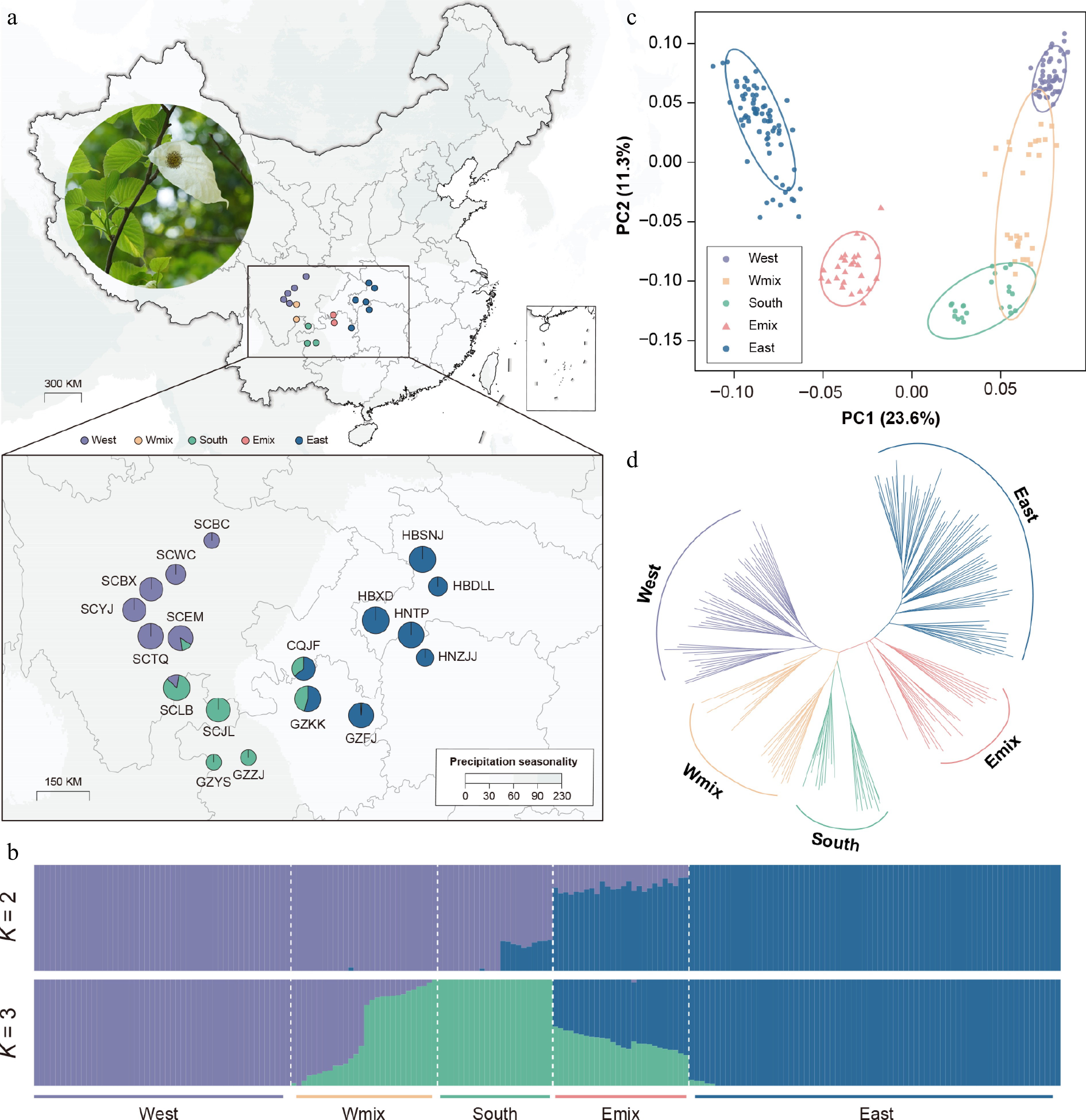
Figure 1. 

Genetic structure, variation, and differentiation of Davidia involucrata. (a) Geographic distribution of 18 natural populations, with a photo of the dove tree. Points with colors represent individual ancestries inferred by the admixture analysis (K = 3). (b) Population assignment using ADMIXTURE with K = 2 and K = 3. The height of each colored segment represents the proportion of the individual ancestries. (c) Principal component analysis (PCA), showing five genetic groups of D. involucrata. (d) The NJ tree of D. involucrata.

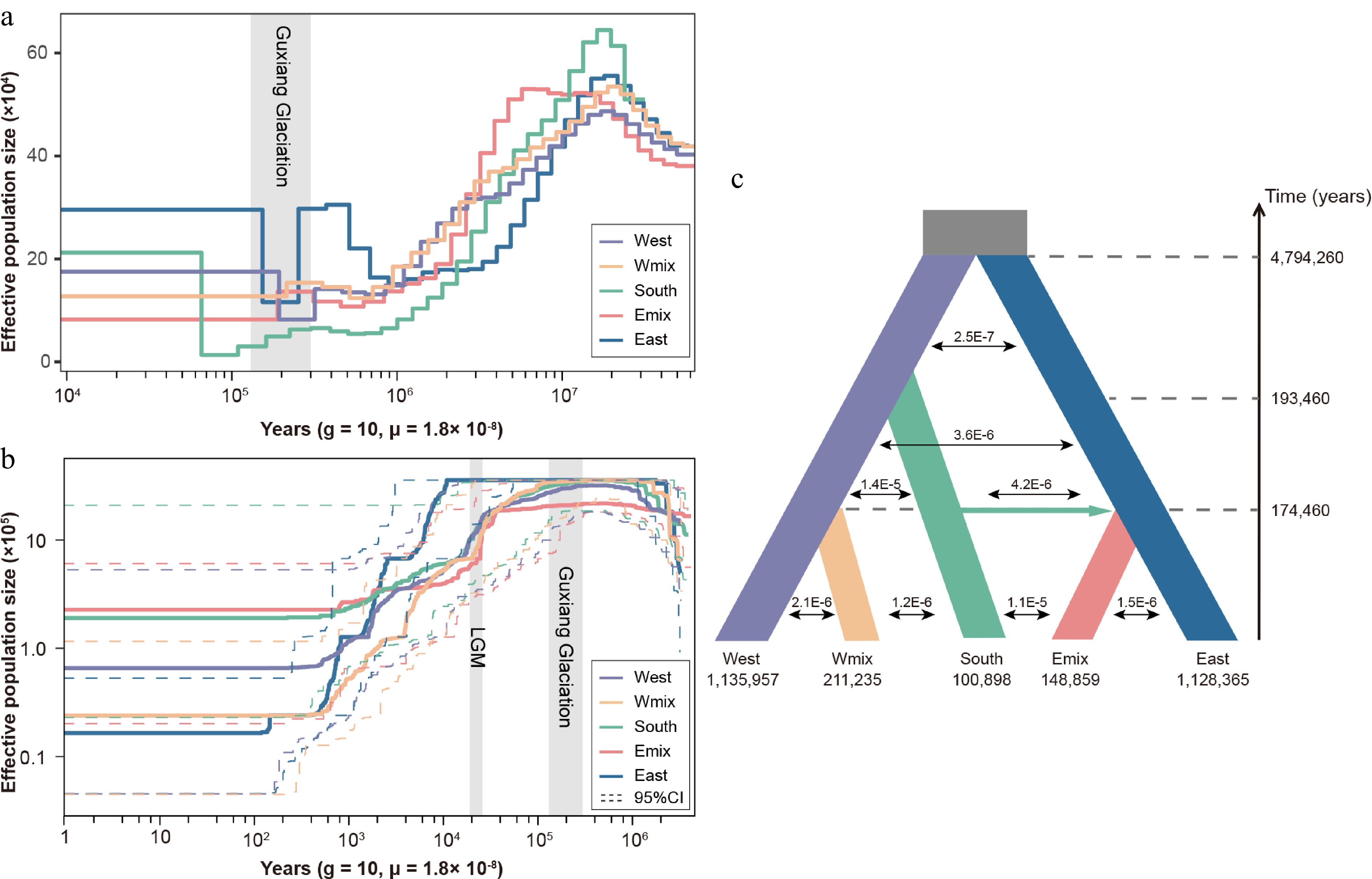
Figure 2. 

Demographic history of three lineages and two admixed groups in Davidia involucrata. (a) Effective population size dynamics inferred by pairwise sequentially Markovian coalescence (PSMC). (b) Effective population size dynamics inferred by StairwayPlot. Dashed lines represent the 95% confidence intervals (c) Divergence times, effective population sizes, and migration rates inferred for Davidia involucrata lineages using fastsimcoal2.7. The grey rectangles refer to the Guxiang glaciation periods and the last glacial maximum (LGM).

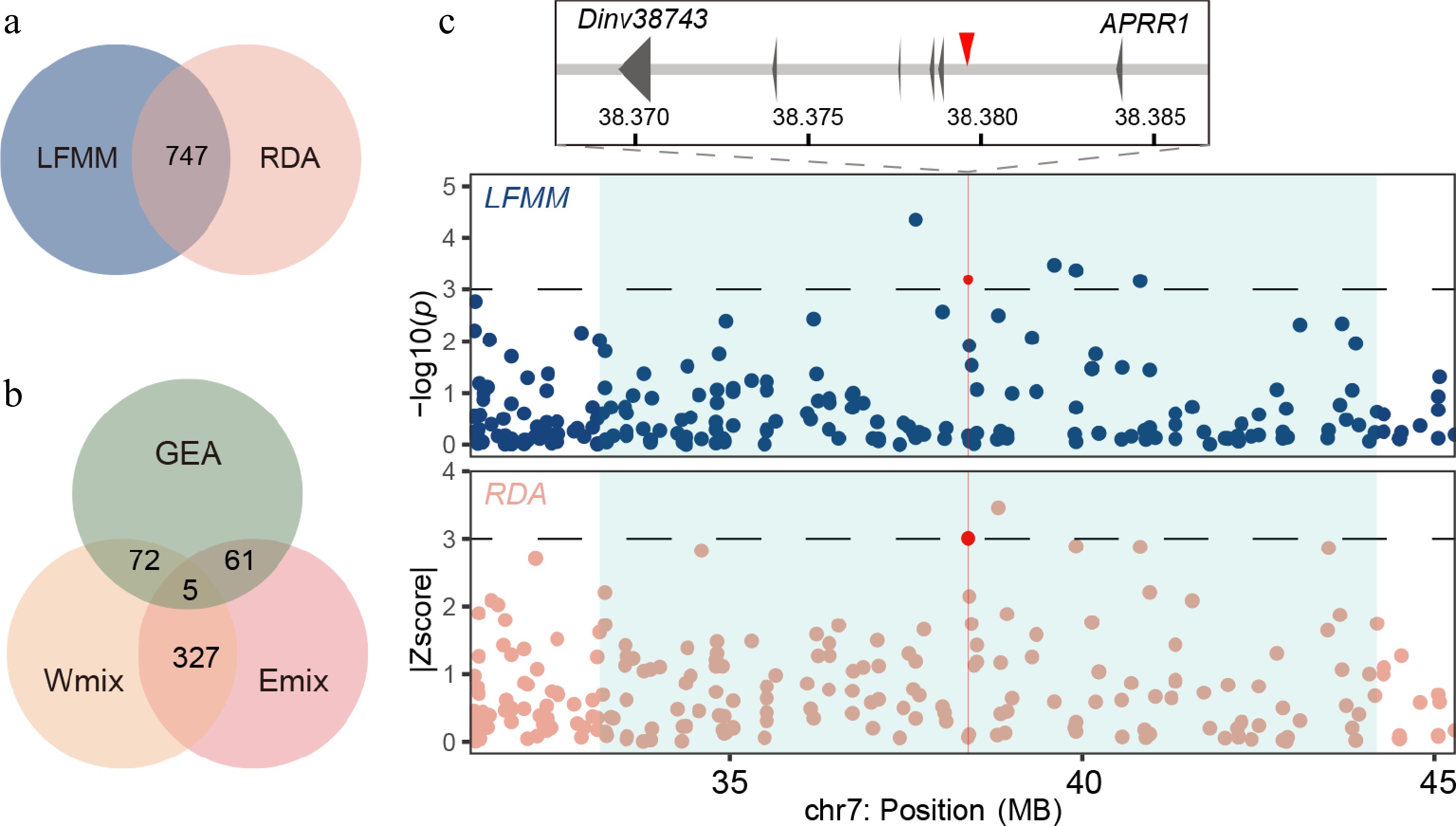
Figure 3. 

Genome-wide screening of the loci associated with local environmental adaptation. (a) Venn plot of outliers from the LFMM analysis and RDA. (b) Venn plot of alleles from GEA outliers and introgressive area of the Emix and Wmix groups. (c) Manhattan plot for variants associated with the seasonality of temperature (BIO4) in the LFMM analysis (upper panel) and the annual precipitation (BIO12) in the RDA (lower panel). Dashed horizontal lines refer to significance thresholds, and red points indicate the significant alleles (chr7: 38379580) in the introgressive area. The introgression windows are shown as light blue rectangles.

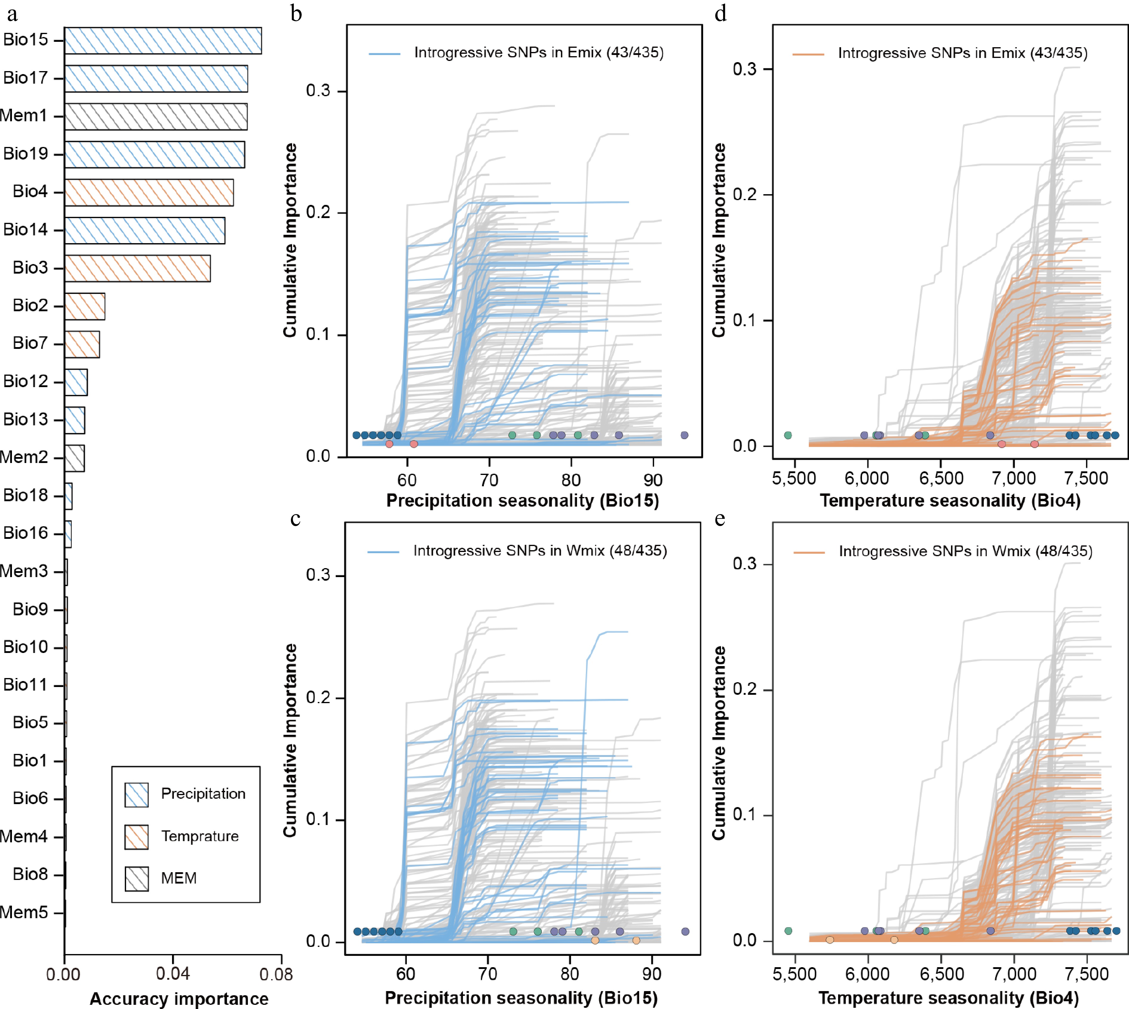
Figure 4. 

Accuracy importance of all predictors and cumulative importance for two variables in the gradient forest model. (a) Importance ranking of all environmental and spatial variables, showing the allelic turnover functions of 435 climate-associated SNPs relative to two high-ranking bioclimatic variables, i.e., seasonality of precipitation (BIO15) and seasonality of temperature (BIO4). Thin lines show each of the 435 candidate SNPs. For BIO15, the introgressive SNPs identified in the Emix (b) and Wmix (c) groups are highlighted in blue. For BIO4, the introgressive SNPs identified in the Emix (d) and Wmix (e) groups are highlighted in orange. Dots represent the environmental variables of 18 sampling sites, with the colors corresponding to the population structure identified in Figure 1.

Figure 5. 

Genomic offset based on GEA outliers for 2081–2100. Local offsets across the range of D. involucrata for SSP245 (a) and SSP585 (b). Violin plot of local offsets in three lineages and two admixed groups for SSP245 (c) and SSP585 (d). The phylogenic tree indicates the relationship of the five genetic groups.

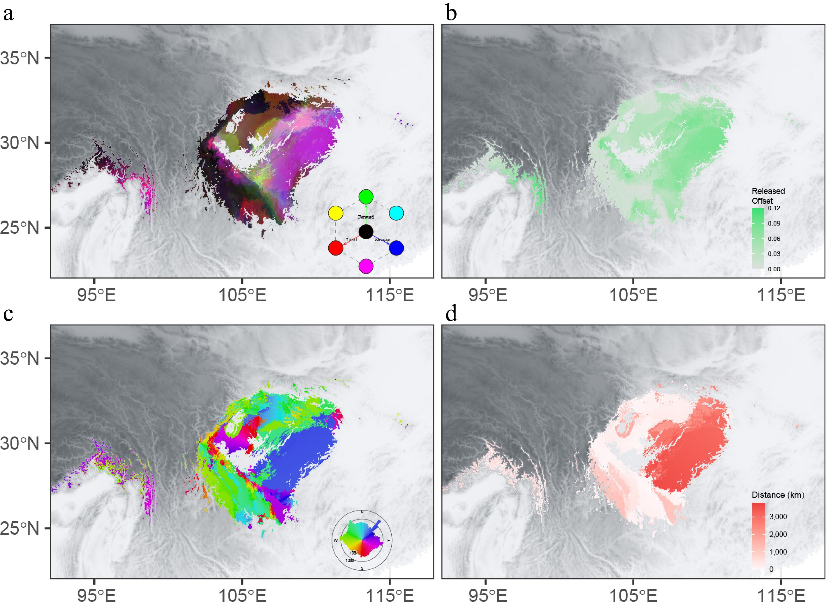
Figure 6. 

Integrated offset, migration distance, and initial bearing for SSP245 in 2081–2100. (a) Mapping of local offsets (red), forward offsets (green), and reverse offsets (blue). (b) The difference between local offsets and forward offsets. The migration distance to (c) and initial bearing (d) of the locations that minimize forward offset.