-
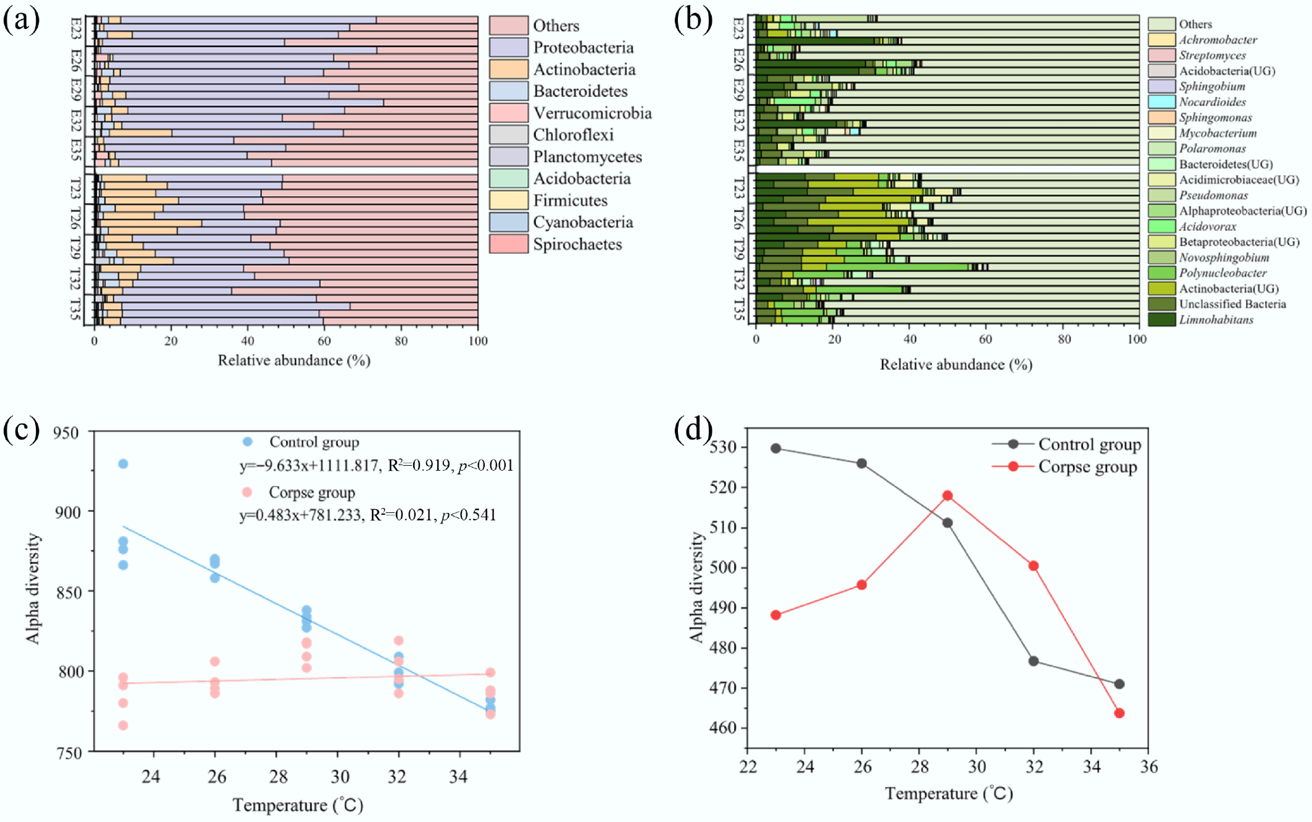
Figure 1.
Carbon cycling bacterial community composition at the (a) phylum, and (b) genus level in the control and experimental groups. Only dominant genera with the top 10 highest mean relative abundance are shown. (c) The result of linear fitting showed the relationship between alpha diversity of CAZy genes and temperature. The results of linear fitting and p value are listed on the figures, and p < 0.05 indicates significant difference. (d) A line chart revealed the change trend of alpha diversity of carbon cycling KO genes. Abbreviations: E, experimental groups; T, control groups.
-
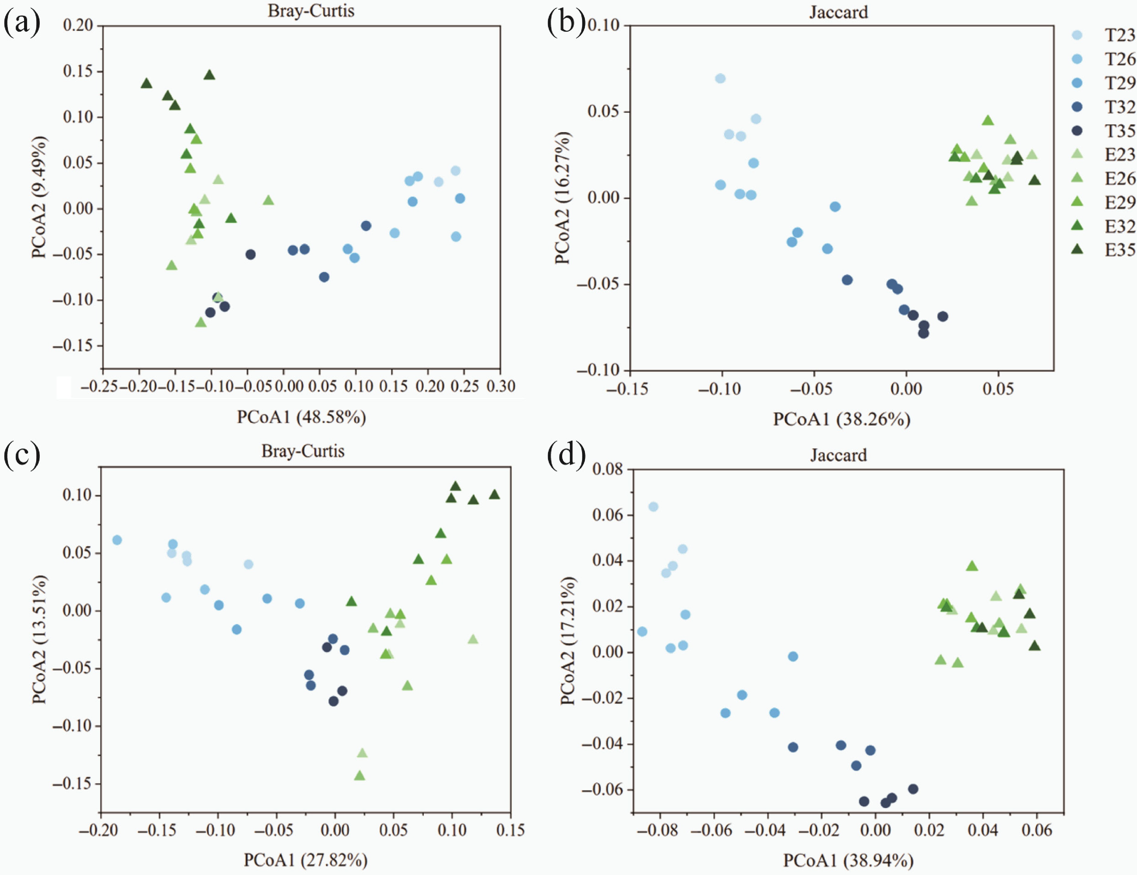
Figure 2.
Principal coordinate analysis (PCoA) of carbon cycling (a), (b) KO, and (c), (d) CAZy genes based on (a), (c) Bray-Curtis, and (b), (d) Jaccard distance matrices. Each point represented the average PCoA values of the corresponding dimension of each group. The blue color represented the control groups, and green represented experimental groups. The color from light to dark reflected the temperature rise. Abbreviations: E, experimental groups; T, control groups.
-
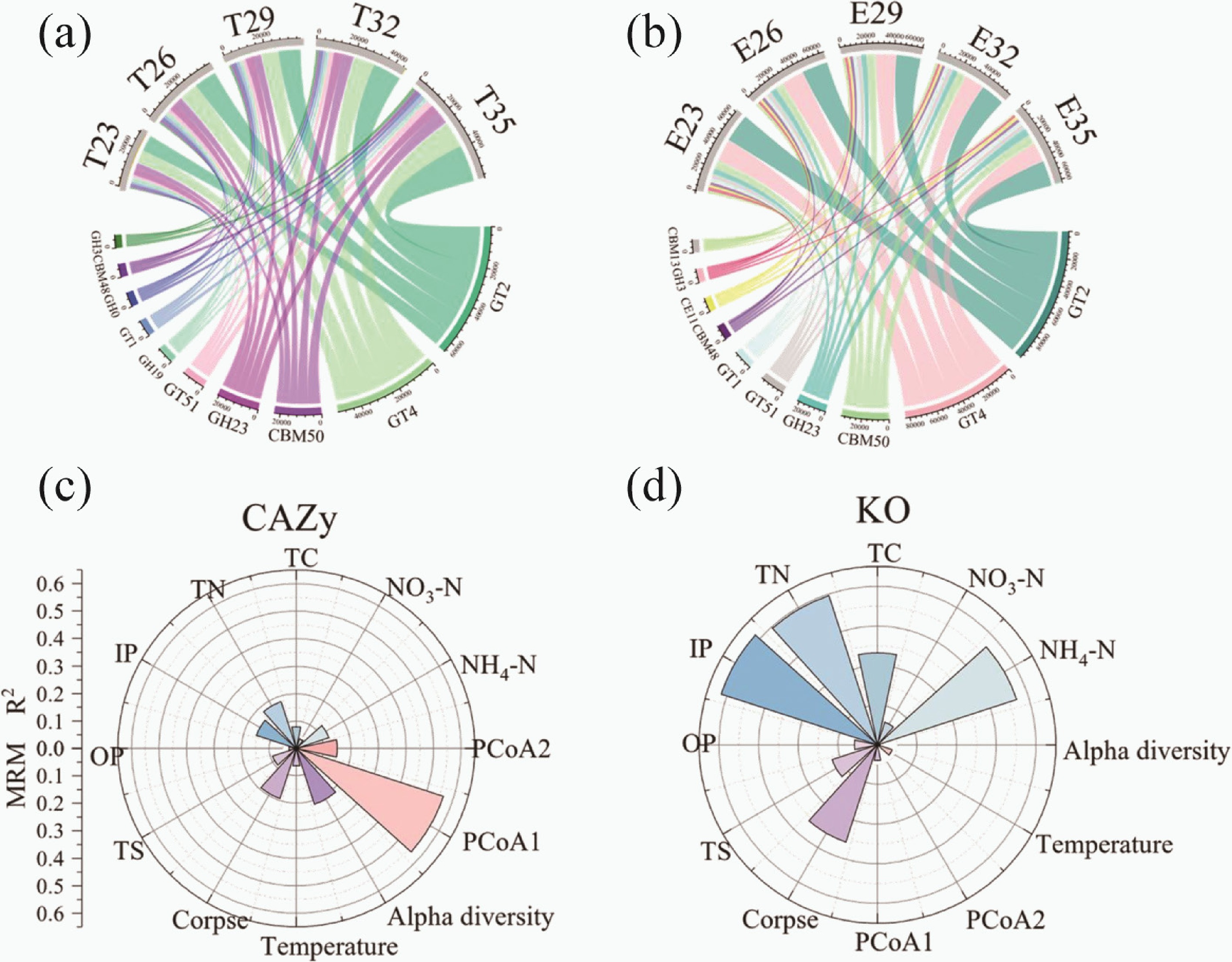
Figure 3.
The chord diagram showed the distribution of the 10 CAZy genes with the highest TPM (transcripts per million) abundance in the (a) control groups, and the (b) experimental groups. Multiple regression matrices (MRM) showing the relative contribution (R2) of these factors for (c) CAZy, and (d) carbon cycling KO genes based on the Bray-Curtis distance metrics. Only the factors with p value < 0.05 are shown. Abbreviations: E, experimental groups; T, control groups; TN, total nitrogen; TC, total carbon; IP, inorganic phosphorus; OP, organic phosphor; TS, total sulphur.
-
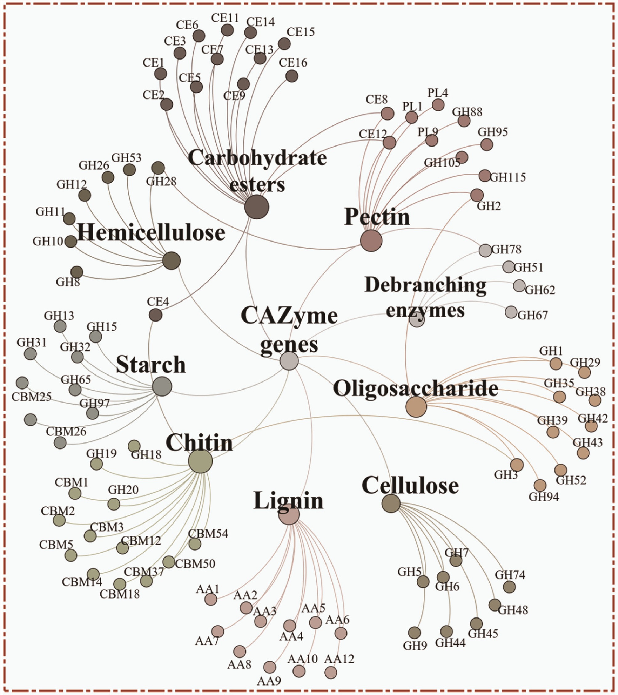
Figure 4.
Network analysis showing the carbohydrate decomposition genes of starch, carbohydrate esters, pectin, lignin, chitin, cellulose, oligosaccharide, debranching enzymes, and hemicellulose.
-
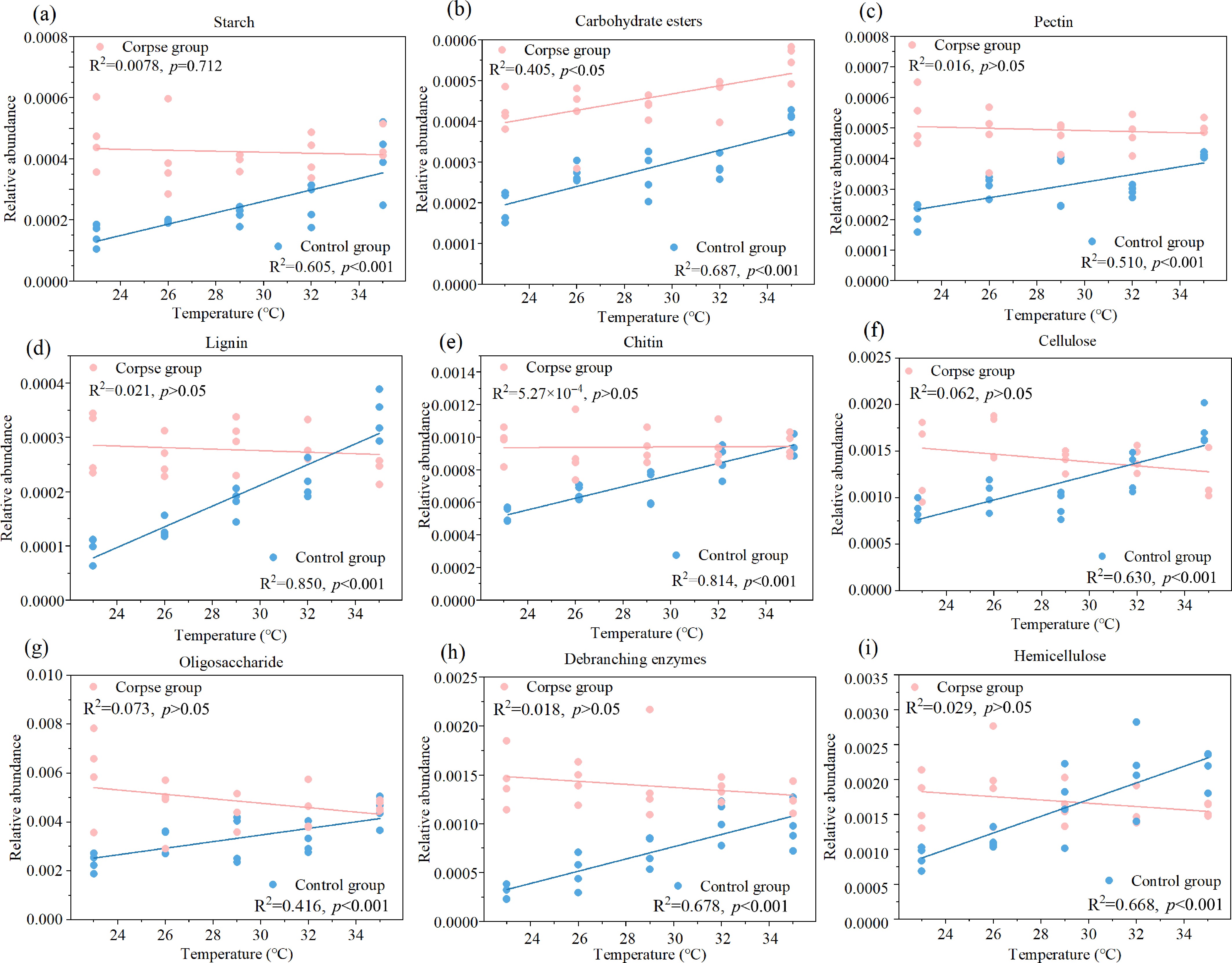
Figure 5.
The linear fitting graphs revealed the interrelationship between relative abundance of nine kinds of carbohydrate decomposition genes—(a) starch; (b) carbohydrate esters; (c) pectin; (d) lignin; (e) chitin; (f) cellulose; (g) oligosaccharide; (h) debranching enzymes; (i) hemicellulose, and temperature in control (blue) and experimental groups (pink). The results of linear fitting and p value were listed on the figures, and p < 0.05 indicates significant difference.
-
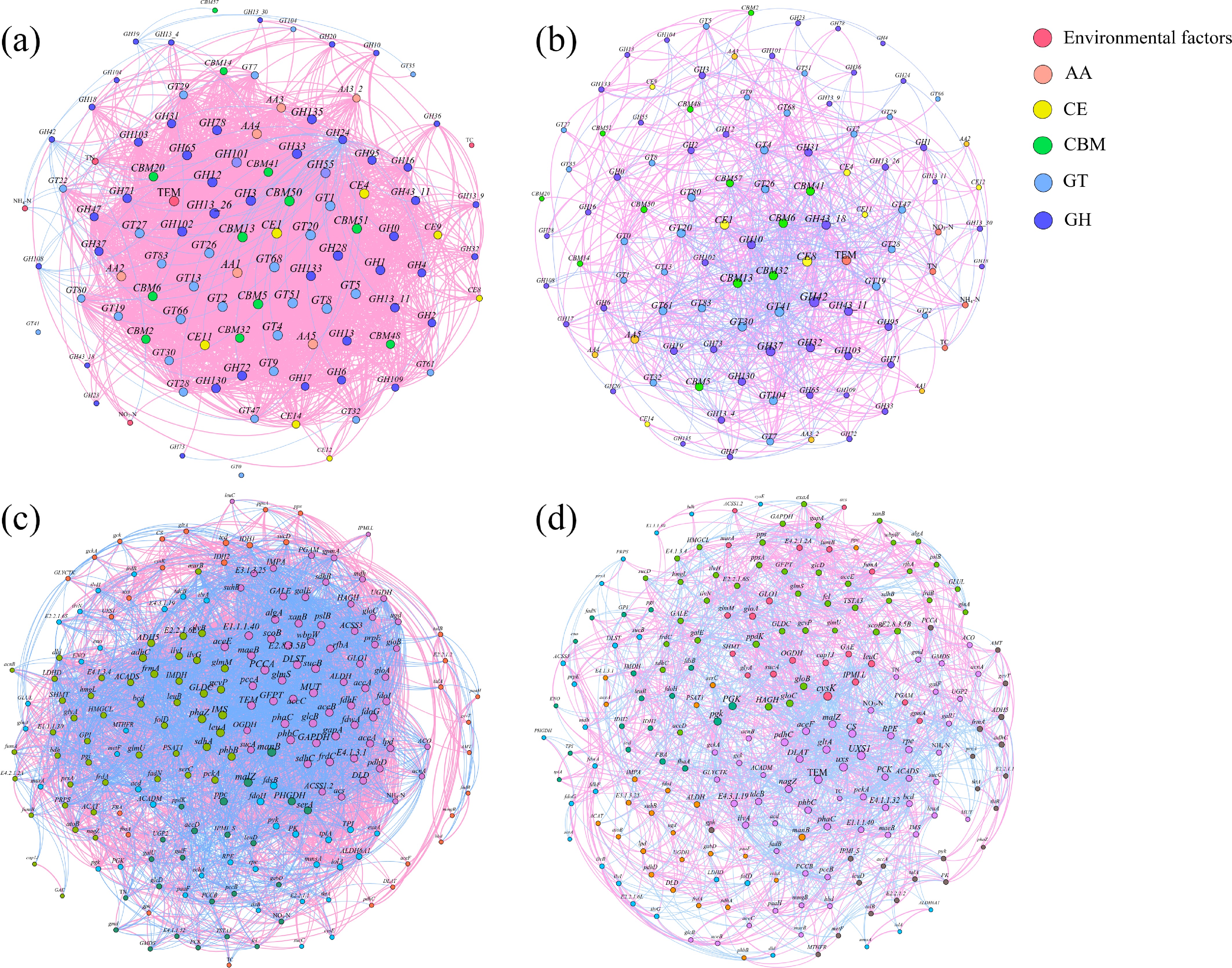
Figure 6.
Co-occurrence network (correlation matrix calculated by R package 'psych', |r| > 0.5, p < 0.05) of (a), (b) CAZy genes, and (c), (d) carbon cycling KO genes in the (a), (c) control, and (b), (d) experimental groups. For the carbon cycling KO genes, the most abundant 200 genes and the physicochemical properties are included. Nodes were colored according to (a), (b) classification, and (c), (d) modularity, and node size represented the correlation between genes. Information on key nodes is nearby the network figures.
-
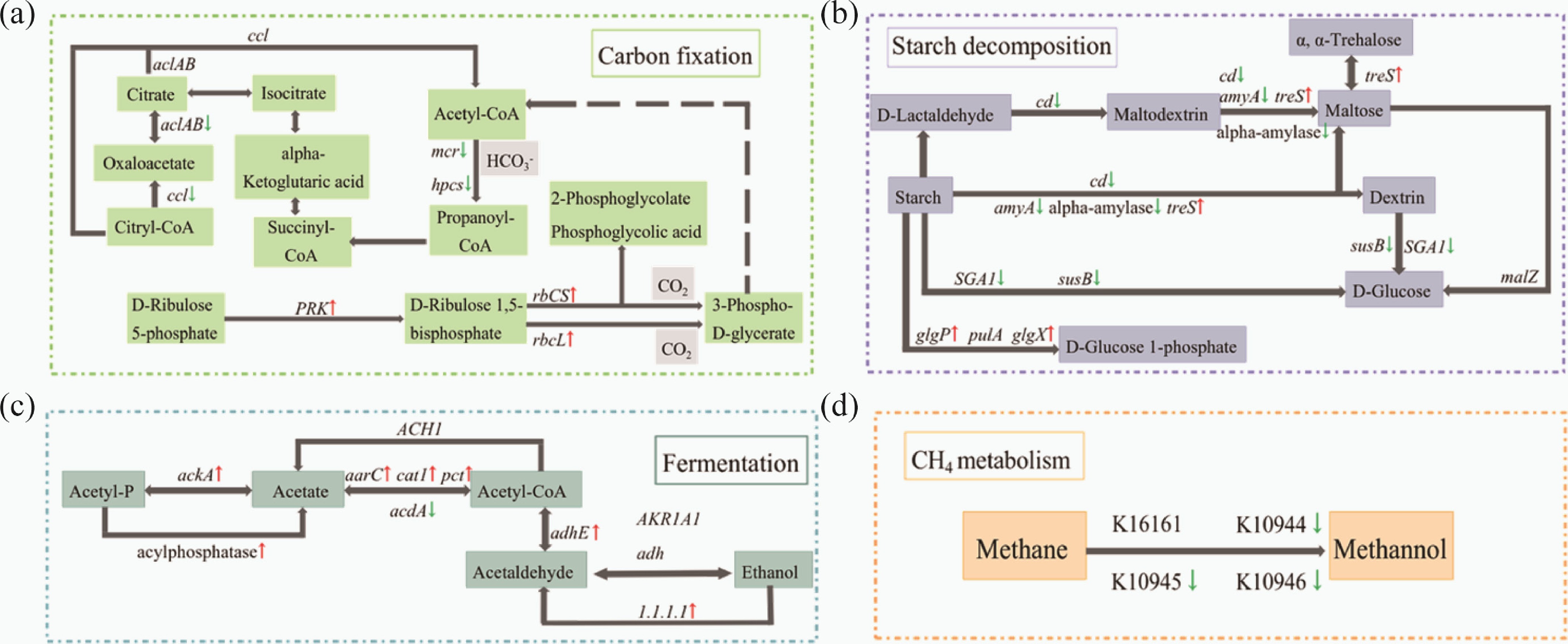
Figure 7.
Flow chart reconstruction of the carbon cycle pathway. (a) carbon fixing; (b) fermentation; (c) starch decomposition; (d) CH4 metabolism. The flow chart shows the genes that were significantly down-regulated (green arrow) or up-regulated (red arrow) in the experimental group, compared with the control group (one-way ANOVA, p < 0.05).
Figures
(7)
Tables
(0)