-
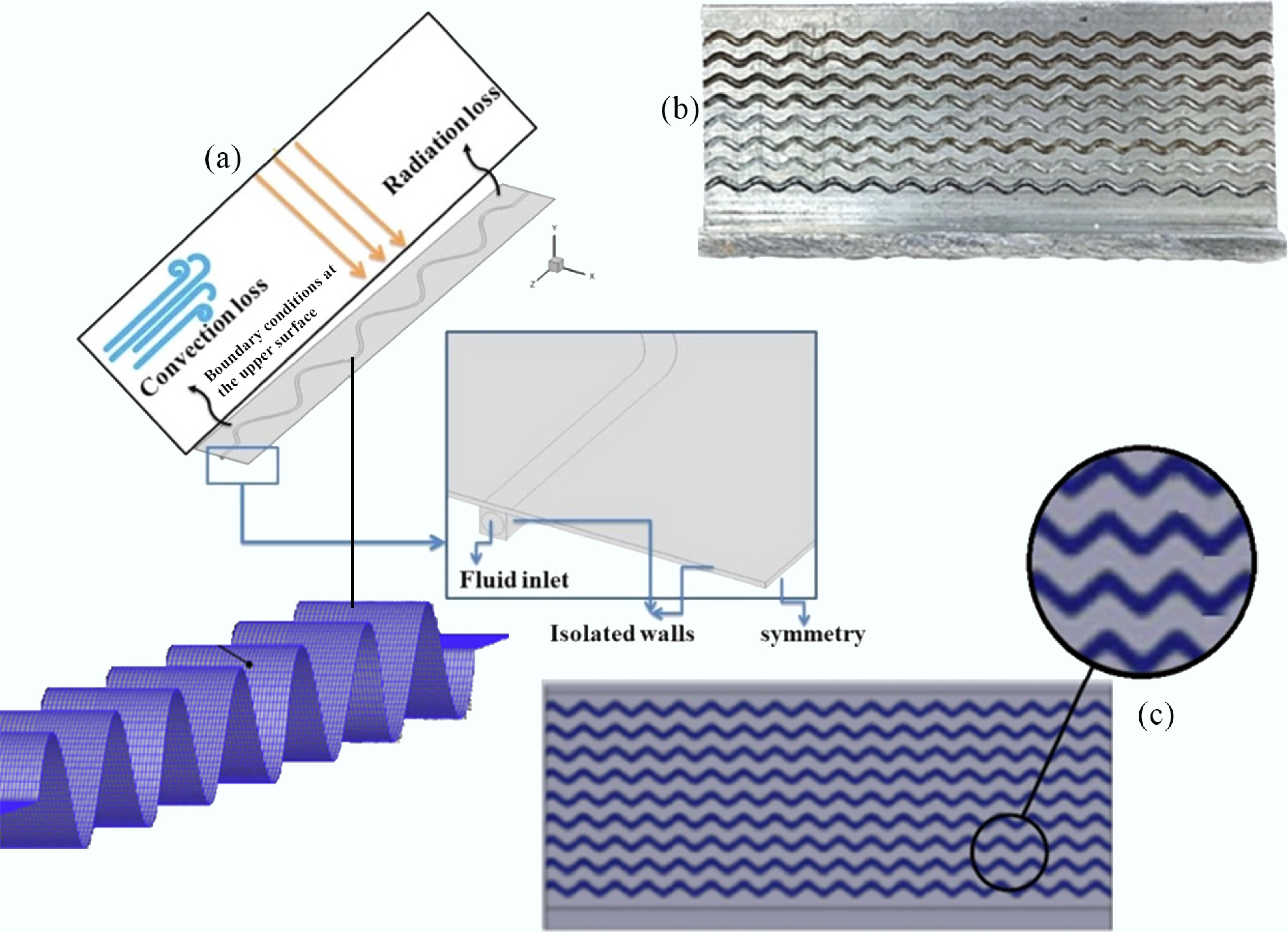
Figure 1.
Schematic representation of the physical model and computational domain with a sinusoidal surface. (a) Heat transfer mechanisms and loss components. (b) Boundary conditions and symmetry setup. (c) Overall system configuration.
-
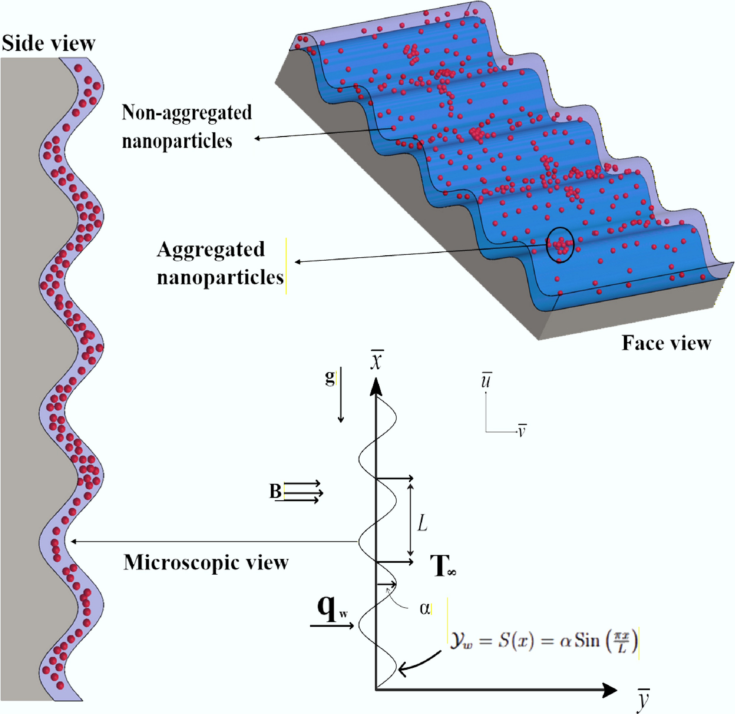
Figure 2.
Geometrical configuration of nanoparticle clustering near a sinusoidal surface.
-
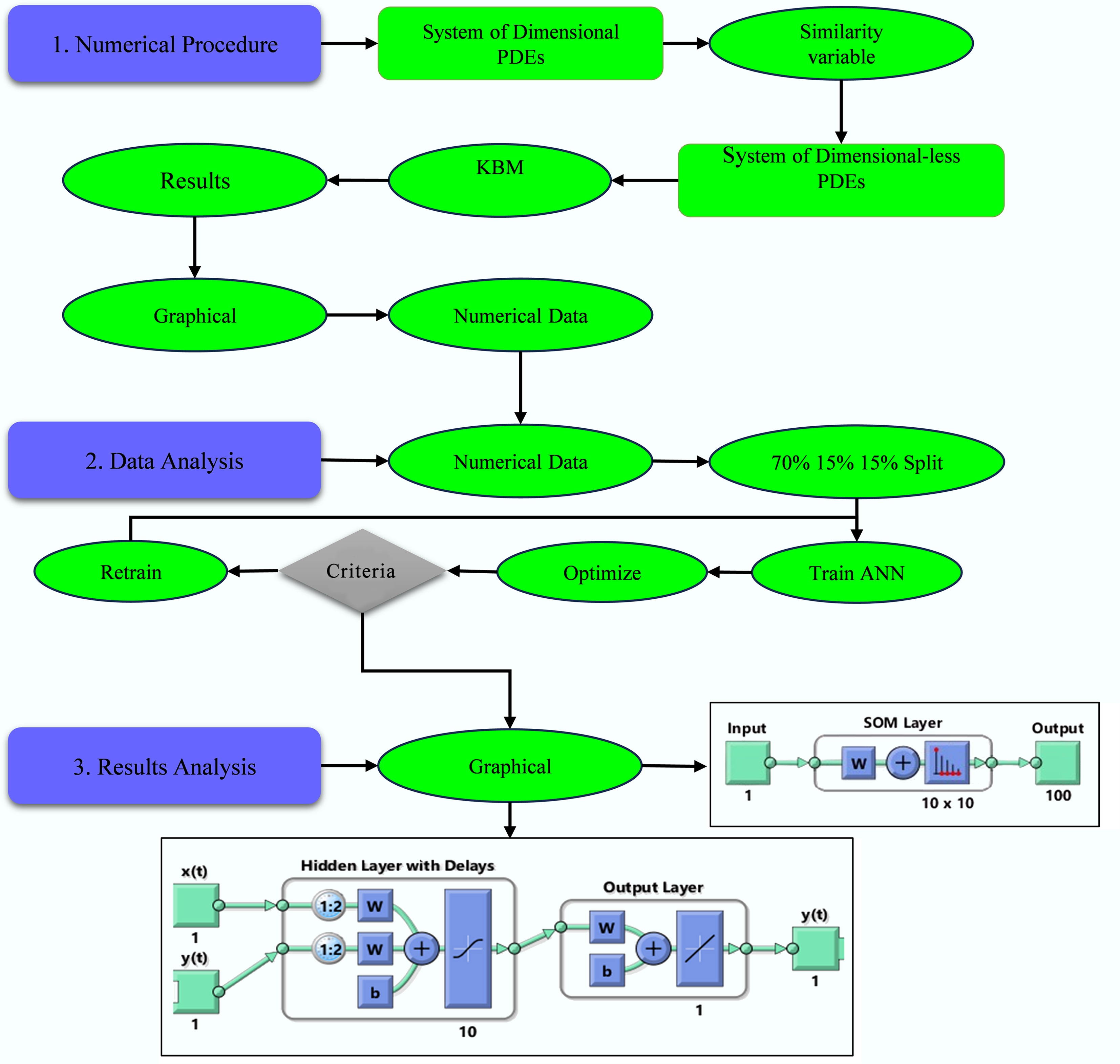
Figure 3.
Computational workflow for Integrated numerical modeling to validate predictions.
-
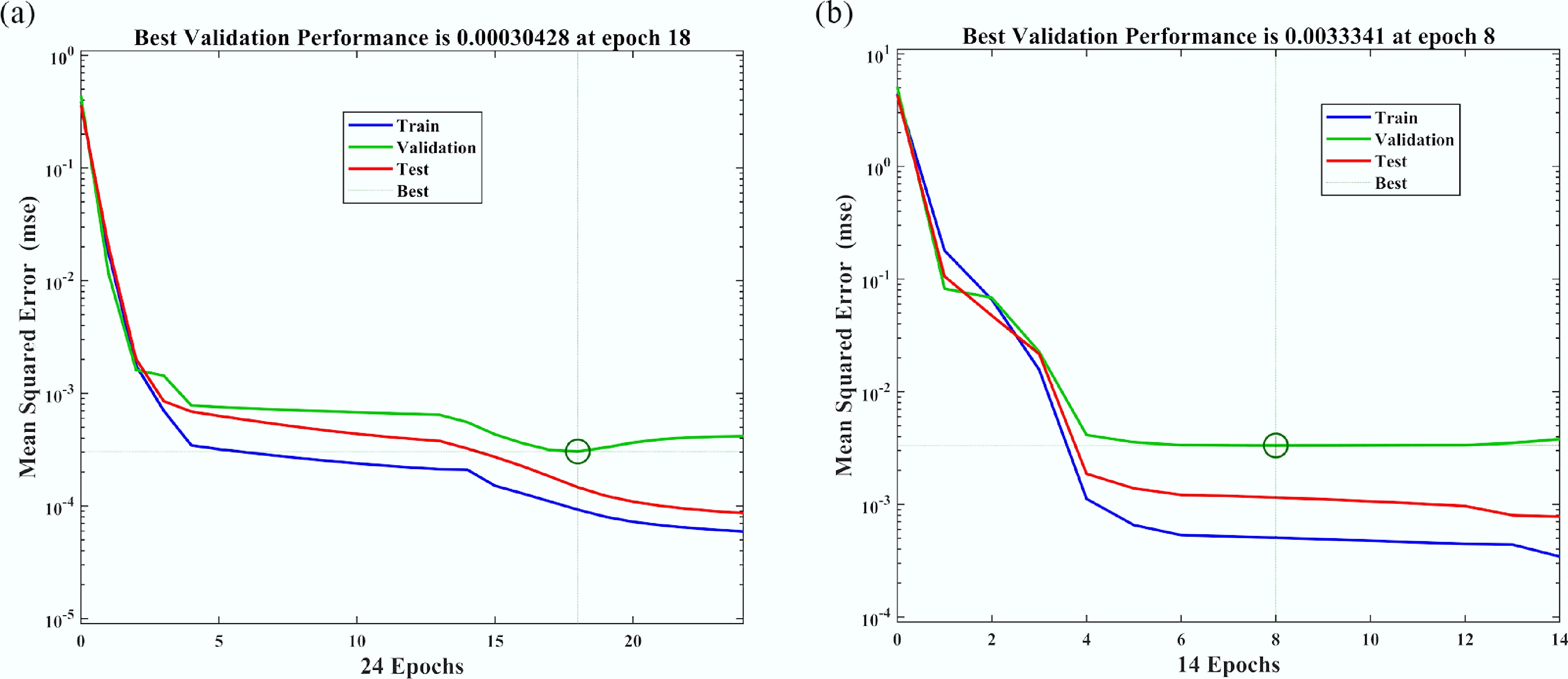
Figure 4.
Mean squared error (MSE) analysis for Nusselt number (Nu) vs sinusoidal parameter (
$ {\varepsilon }_{T} $ -
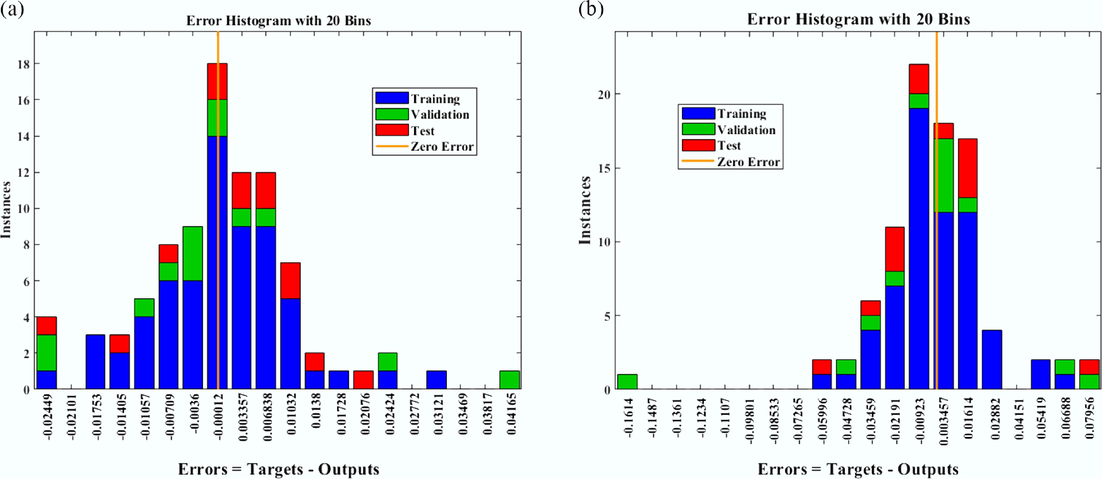
Figure 5.
Error histogram analysis for Nusselt number (Nu) vs sinusoidal parameter (
$ {\varepsilon }_{T} $ -
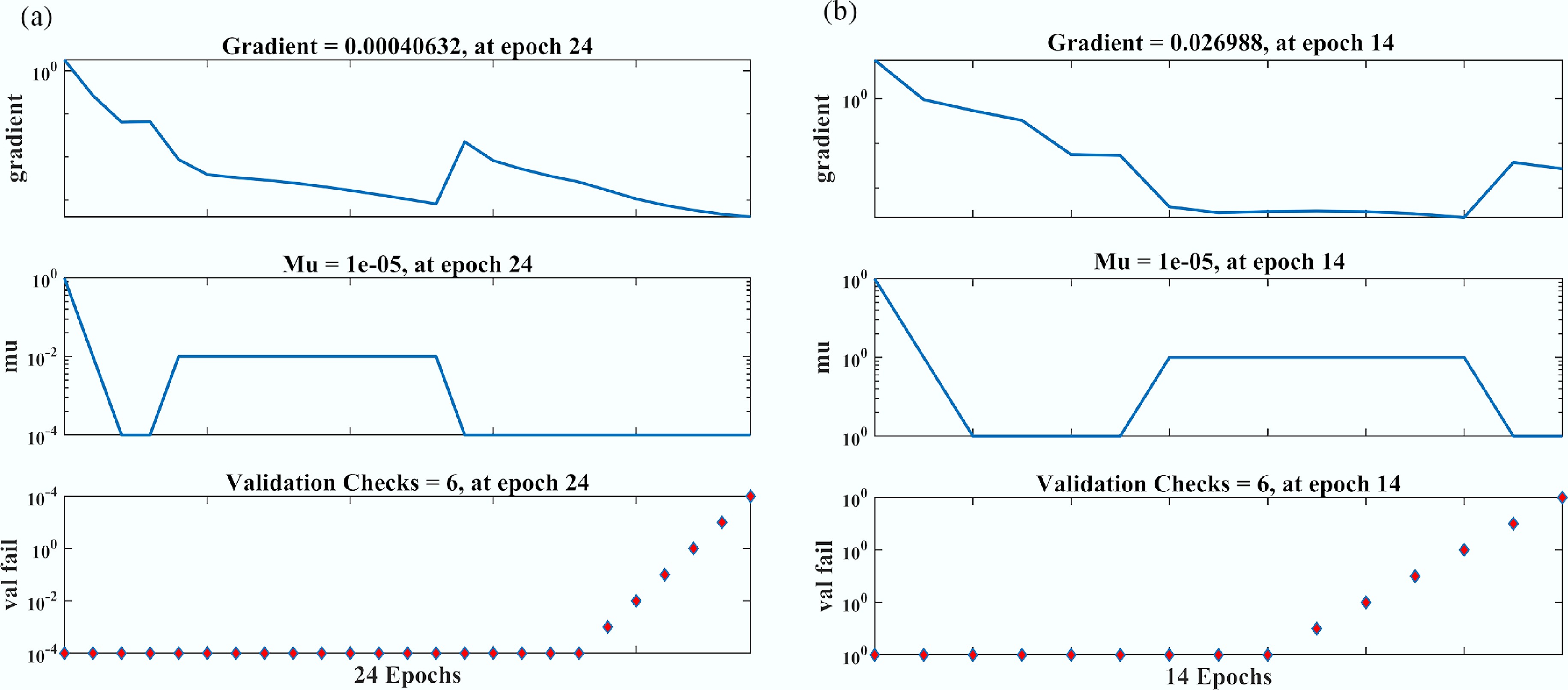
Figure 6.
Gradient validation analysis for Nusselt number (Nu) vs sinusoidal parameter (
$ {\varepsilon }_{T} $ -
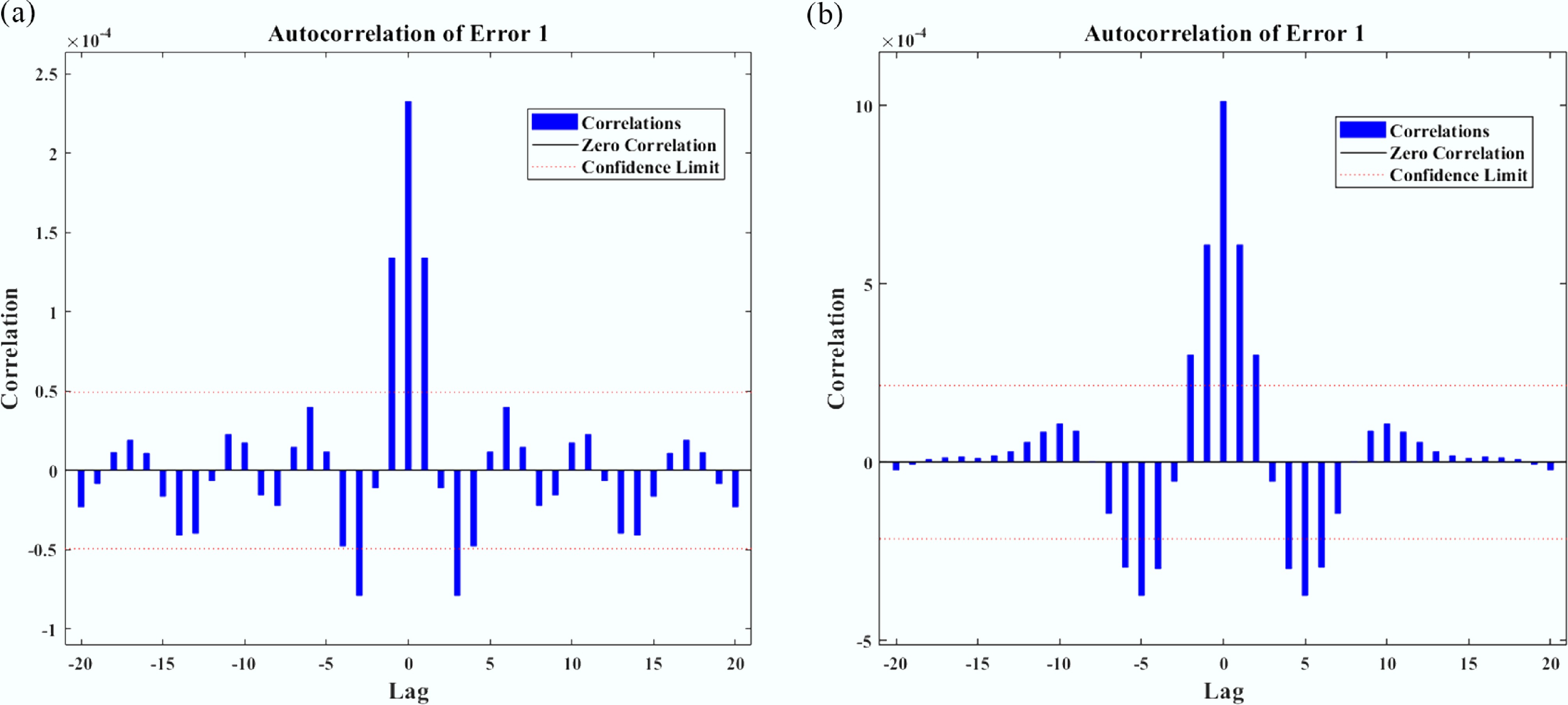
Figure 7.
Correlation patterns analysis for Nusselt number (Nu) vs sinusoidal parameter (
$ {\varepsilon }_{T} $ -
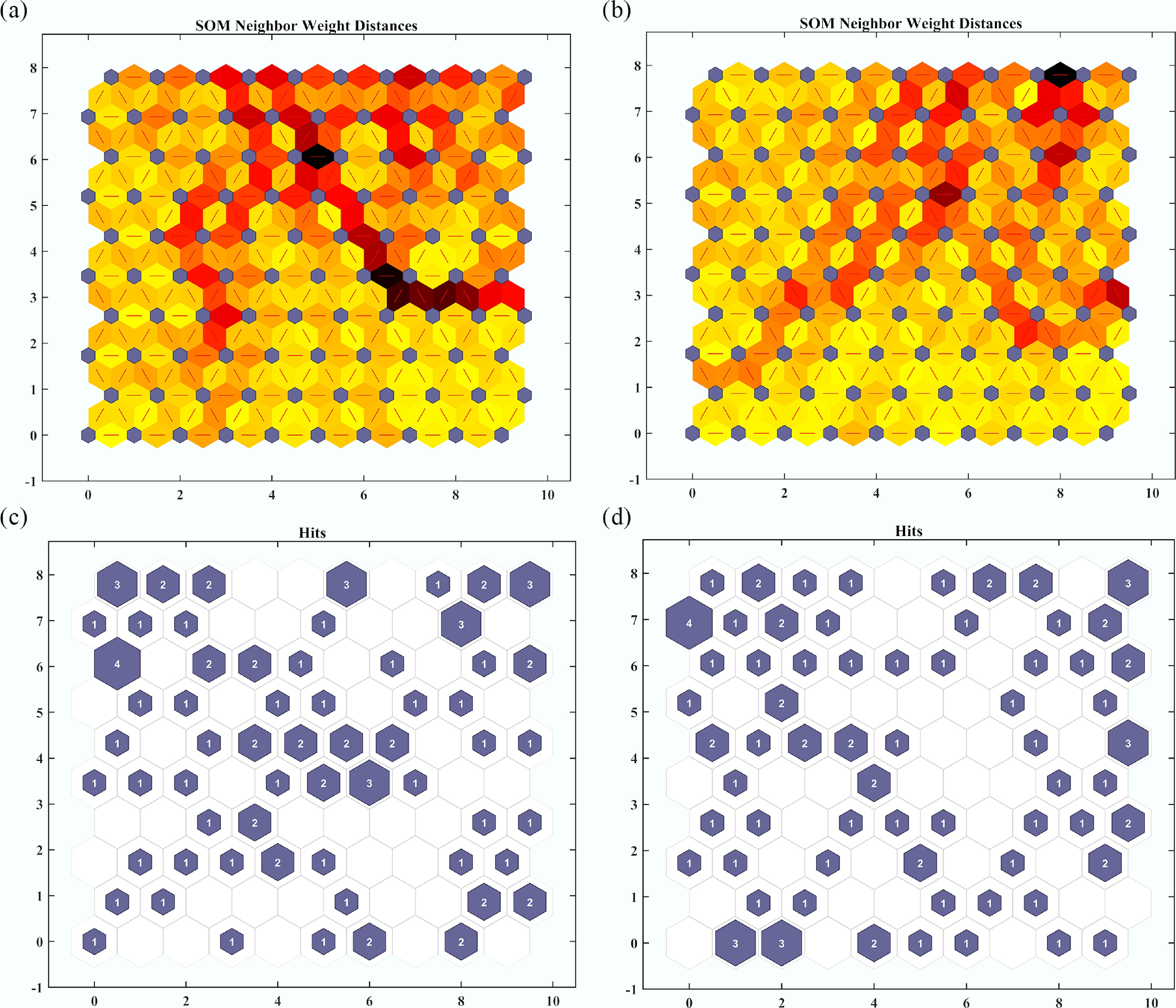
Figure 8.
Clustering analysis of the Nusselt number (Nu) as a function of the sinusoidal parameter (
$ {\varepsilon }_{T} $ -
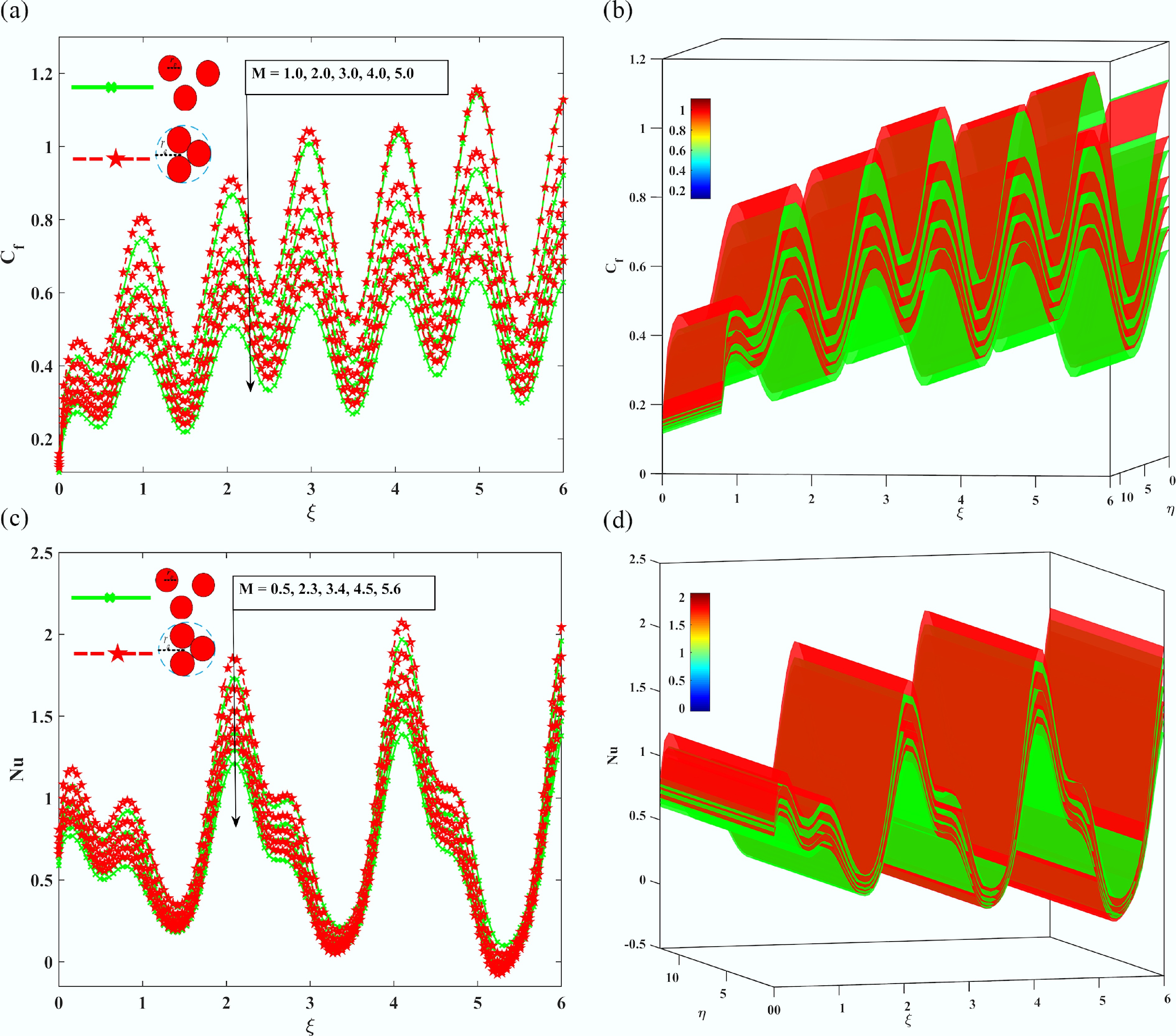
Figure 9.
The Impact of the magnetic parameter M, on (a), (b) skin friction coefficient Cf, and (c), (d) local Nusselt number Nu.
-
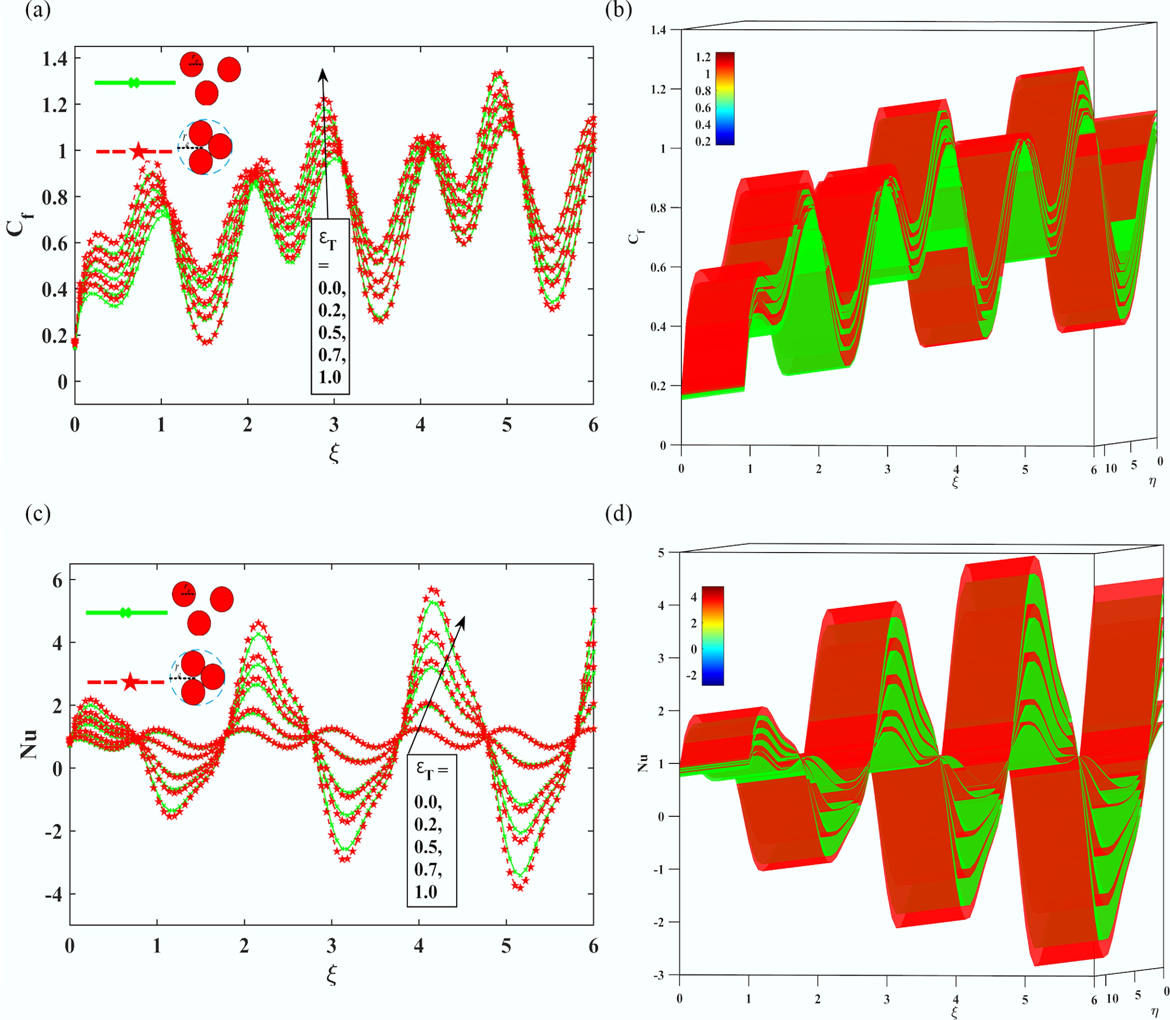
Figure 10.
The Impact of sinusoidal boundary parameter
$ {\varepsilon }_{T} $ -
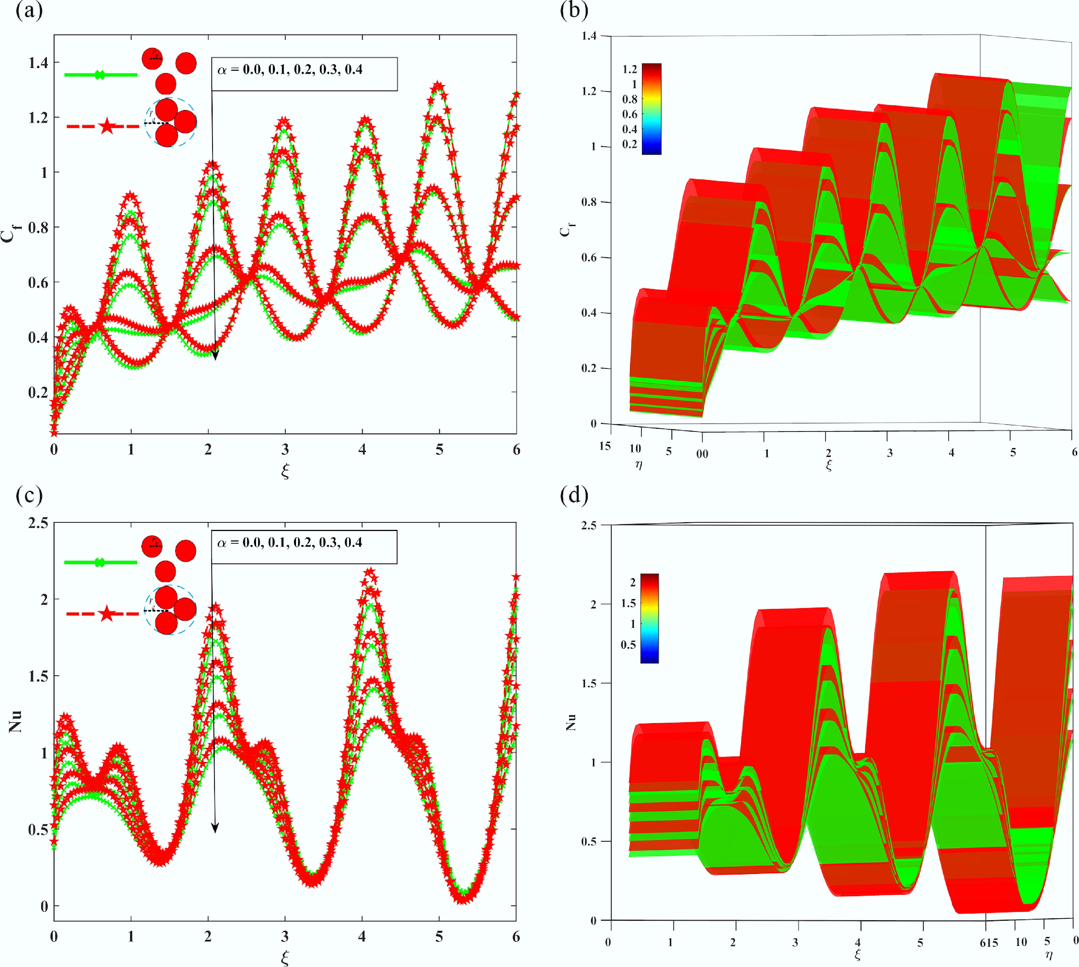
Figure 11.
The Impact of the wavelength ratio parameter
$ \alpha $ -
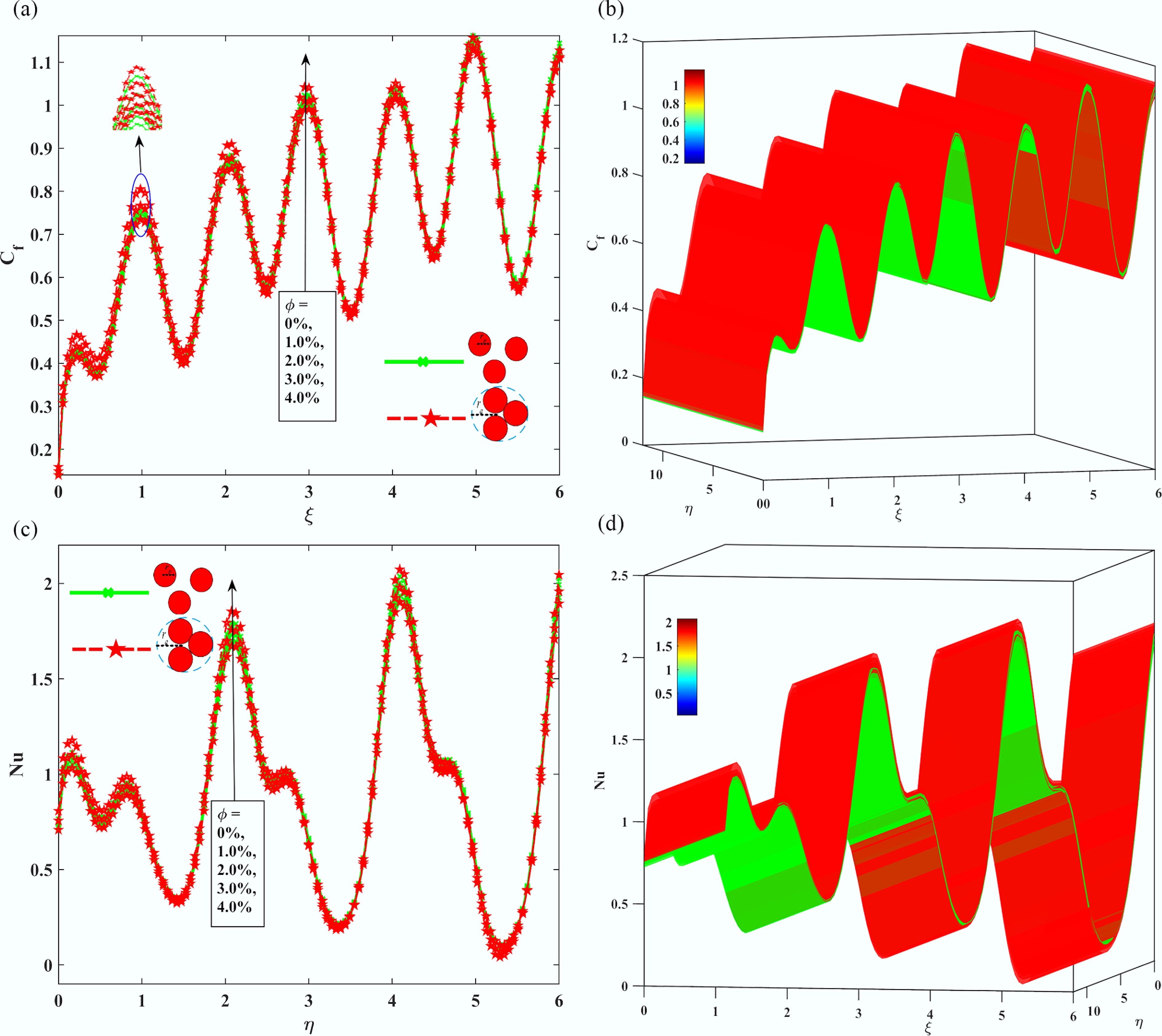
Figure 12.
The Impact of the concentration of NP
$ \phi $ -
Property Constant Non-aggregation Aggregated Viscosity $ \mu $ D1 $ {\mu }_{n f}={\mu }_{f}{\left(1-\varphi \right)}^{-2.5} $ $ {\mu }_{n f}={\mu }_{f}{\left(\dfrac{{\phi }_{m}-{\phi }_{a}}{{\phi }_{m}}\right)}^{{{\phi }_{m}}} $ Density $ \rho $ D2 $ {\rho }_{n f}={\rho }_{f}\left[\left(1-\phi \right)+\phi \left(\dfrac{{\rho }_{s}}{{\rho }_{f}}\right)\right] $ $ {\rho }_{n f}={\rho }_{f}\left[\left(1-{\phi }_{a}\right)+{\phi }_{a}\left(\dfrac{{\rho }_{s}}{{\rho }_{f}}\right)\right] $ Specific heat capacity Cp D3 $ {\left(\rho {C}_{P}\right)}_{nf}={\left(\rho {C}_{P}\right)}_{f}\left[\left(1-\phi \right)+\dfrac{{\left(\rho {C}_{P}\right)}_{s}}{{\left(\rho {C}_{P}\right)}_{f}}\phi \right] $ $ {\left(\rho {C}_{P}\right)}_{nf}={\left(\rho {C}_{P}\right)}_{f}\left[\left(1-{\phi }_{a}\right)+\dfrac{{\left(\rho {C}_{P}\right)}_{s}}{{\left(\rho {C}_{P}\right)}_{f}}{\phi }_{a}\right] $ Thermal conductivity k D4 $ {k}_{n f}=\left[\dfrac{\left({k}_{s}+2{k}_{f}\right)-2\phi \left({k}_{f}-{k}_{s}\right)}{\left({k}_{s}+2{k}_{f}\right)+\phi \left({k}_{f}-{k}_{s}\right)}\right]{k}_{f} $ $ {k}_{n f}=\left[\dfrac{\left({k}_{s}+2{k}_{f}\right)-2{\phi }_{a}\left({k}_{f}-{k}_{s}\right)}{\left({k}_{s}+2{k}_{f}\right)+{\phi }_{a}\left({k}_{f}-{k}_{s}\right)}\right]{k}_{f} $ Electrical conductivity $ \sigma $ D5 $ {\sigma }_{n f}={\sigma }_{f}+{\sigma }_{f}\left[\dfrac{3\left(\dfrac{{\sigma }_{s}}{{\sigma }_{f}}-1\right)\phi }{\left(\dfrac{{\sigma }_{s}}{{\sigma }_{f}}+2\right)-\left(\dfrac{{\sigma }_{s}}{{\sigma }_{f}}-1\right)\phi }\right] $ $ {\sigma }_{n f}={\sigma }_{f}+{\sigma }_{f}\left[\dfrac{3\left(\dfrac{{\sigma }_{s}}{{\sigma }_{f}}-1\right){\phi }_{a}}{\left(\dfrac{{\sigma }_{s}}{{\sigma }_{f}}+2\right)-\left(\dfrac{{\sigma }_{s}}{{\sigma }_{f}}-1\right){\phi }_{a}}\right] $ Table 1.
Thermophysical properties of aggregated and non-aggregated nanoparticles by Mahanthesh et al.[36]
-
A. Non-aggregated B. Aggregated Scenario Case Selected parameters M $ {\boldsymbol\varepsilon }_{\boldsymbol T} $ Description I (A, B) 1 1 0.5 Weak magnetism over a wavy boundary 2 2 0.5 Moderate field, typical in electronics cooling 3 3 0.5 High-intensity field (advanced heat exchangers) II (A, B) 1 4 1 Flat surface (baseline waviness) 2 4 2 Moderate waviness boosts fluid mixing 3 4 3 High undulation resembling turbulence Table 2.
Parameter sets for scenario construction
-
Property Base fluid Nanoparticle Pure water Diamond $ \mu $ 0.000803 − Density $ \rho $ 997.1 3,510 Specific heat capacity Cp (J/kg·K) 6.13 × 10⁻¹ 497.26 Thermal conductivity k (W/m·K) 4,179 1,000 Average size − 30 nm Range − 20–50 nm Purity − > 95% Table 3.
Thermophysical properties of the considered nanoparticles by Sundar et al.[39]
-
Number of grid points Output η- direction
(With fixed η = 20)ξ- direction
(With fixed ξ = 1)Cf Nu 100 10 −0.85351 0.31688 200 20 −0.85381 0.31699 400 50 −0.85392 0.31680 800 100 −0.85392 0.31680 1,600 200 −0.85382 0.31680 Table 4.
Grid independence test for
$ \phi $ $ \alpha $ -
Scenario Case MSE data Performance Gradient Mu Final epoch Time (s) Training Validation Testing Non-aggregated I A 1 1.48882e–5 3.23527e–5 1.38677e–5 1.21e–5 1.00e–7 1e10 25 < 1 2 1.48550e–5 3.32879e–5 1.47673e–5 1.20e–5 1.92e–8 1e10 67 < 2 3 1.72843e–5 3.13655e–5 1.32171e–5 1.03e–5 1.98e–7 1e10 99 < 3 II A 1 4.35370e–6 4.65936e–5 4.34532e–5 4.09e–6 9.99e–08 1e–6 93 6 2 4.89685e–6 4.54796e–5 4.58981e–5 3.89e–6 9.92e–08 1e–6 104 4 3 4.52364e–6 4.85467e–5 5.41256e–5 4.89e–6 9.98e–08 1e–6 186 3 Aggregated I B 1 2.18093e−7 8.82690e−7 1.22922e−6 1.54e−7 2.50e−5 1e−10 117 3 2 2.18767e−7 8.47592e−7 1.59921e−6 1.73e−7 2.94e−6 1e−10 184 2 3 2.79081e−7 8.85570e−7 2.58671e−6 1.95e−7 3.35e−5 1e−10 220 3 II B 1 5.05758e−4 3.33414e−3 1.15199e−3 4.43e−4 7.33e−7 1e−5 14 2 2 5.05423e−4 3.53341e−3 1.15171e−3 4.55e−4 7.90e−8 1e−5 25 4 3 5.06846e−4 3.69321e−3 1.16161e−3 4.68e−4 7.94e−8 1e−5 46 3 Table 5.
Outcomes of all scenarios with ANNs and LMT
Figures
(12)
Tables
(5)