-
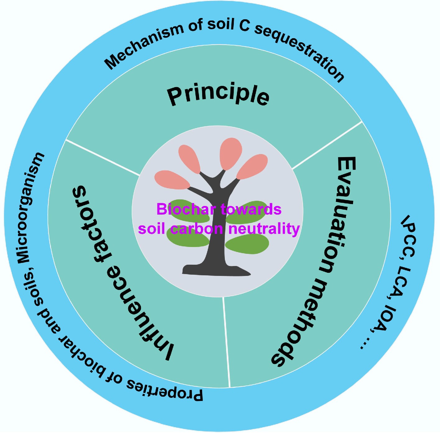
Figure 1.
Schematic illustration of biochar used for soil carbon neutralization.
-
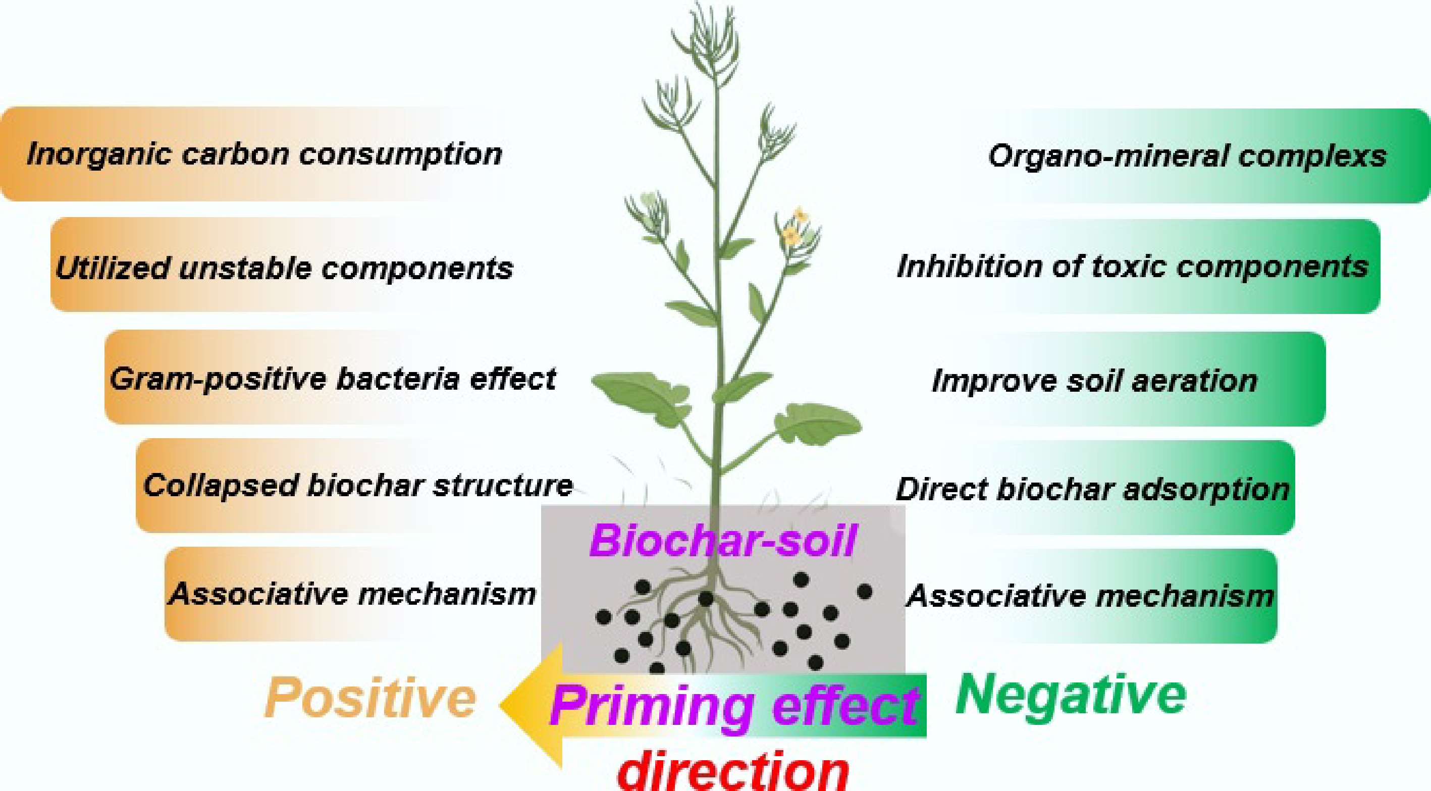
Figure 2.
Schematic diagram of priming effect in biochar-soil system.
-
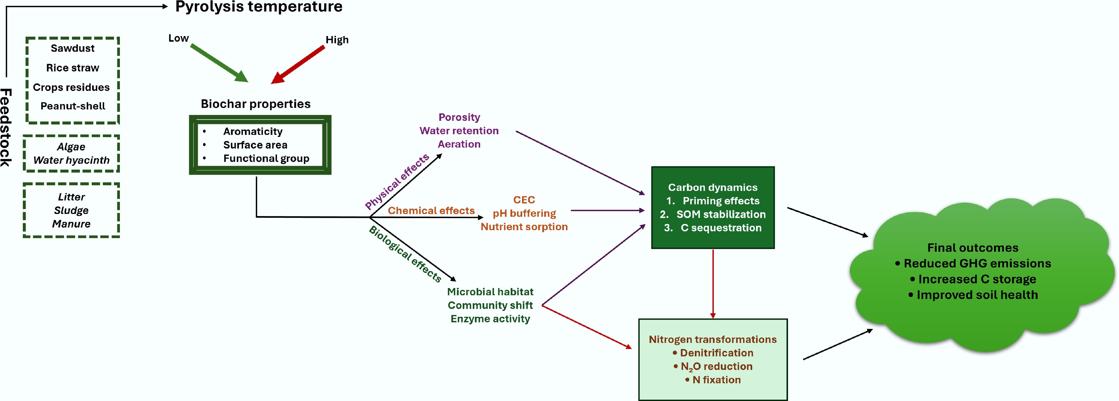
Figure 3.
The effects of feedstock and pyrolysis temperature on biochar properties and its applications impacting soil properties regulating the soil health and GHG emissions.
-
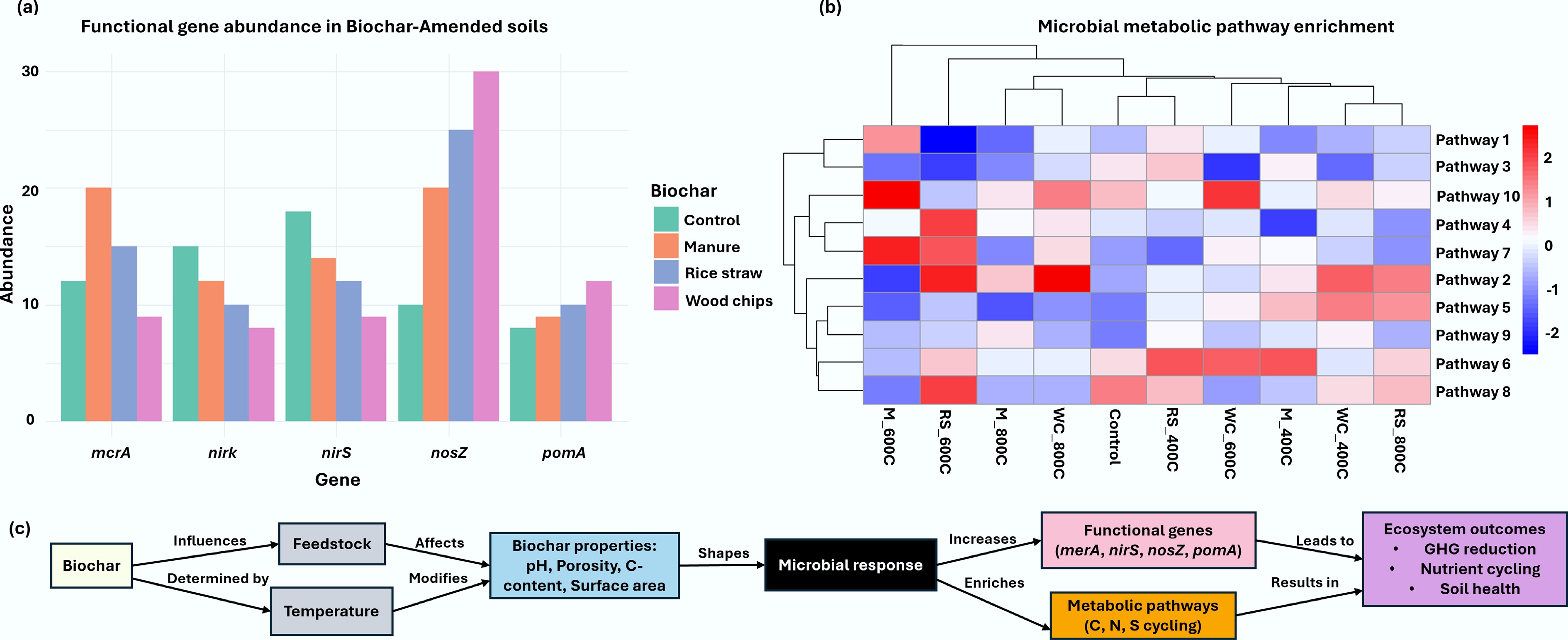
Figure 4.
Microbial functional gene abundance and metabolic pathway enrichment in biochar-amended soils relative to other organic amendments. (a) Synthesis of published studies shows that biochar amendment significantly increases the mean abundance of key functional genes for mercury reduction (merA), denitrification (nirK, nirS, nosZ), and methane oxidation (pmoA) compared to manure, rice straw, wood chips, and unamended control soils. (b) Enrichment of microbial metabolic pathways—including those for carbon fixation, nitrogen metabolism, and aromatic compound degradation—varies with biochar type, defined by feedstock (e.g., maize straw, wheat straw, wood chips, peanut shells) and pyrolysis temperature (400 vs 800 °C). Higher temperature biochar (800 °C) generally induce distinct metabolic profiles compared to those produced at 400 °C, reflecting how feedstock properties and pyrolysis conditions shape microbial functional potential in amended soils. (c) Mechanistic pathways of biochar in assisting microbial growth.
-
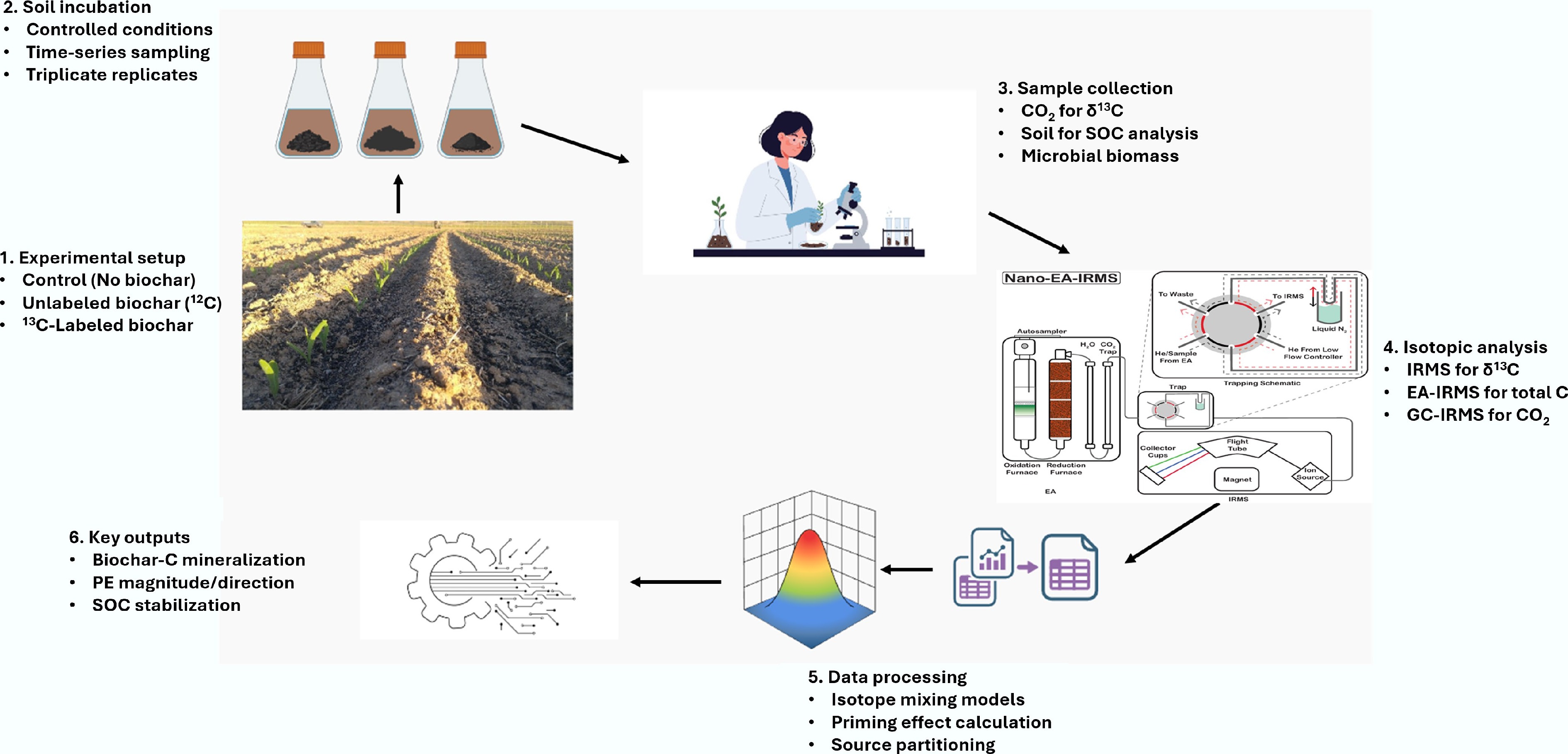
Figure 5.
An illustration depicting the data flow diagram elucidating the experimental procedure and data processing pathway for the 13C-labeled biochar.
-
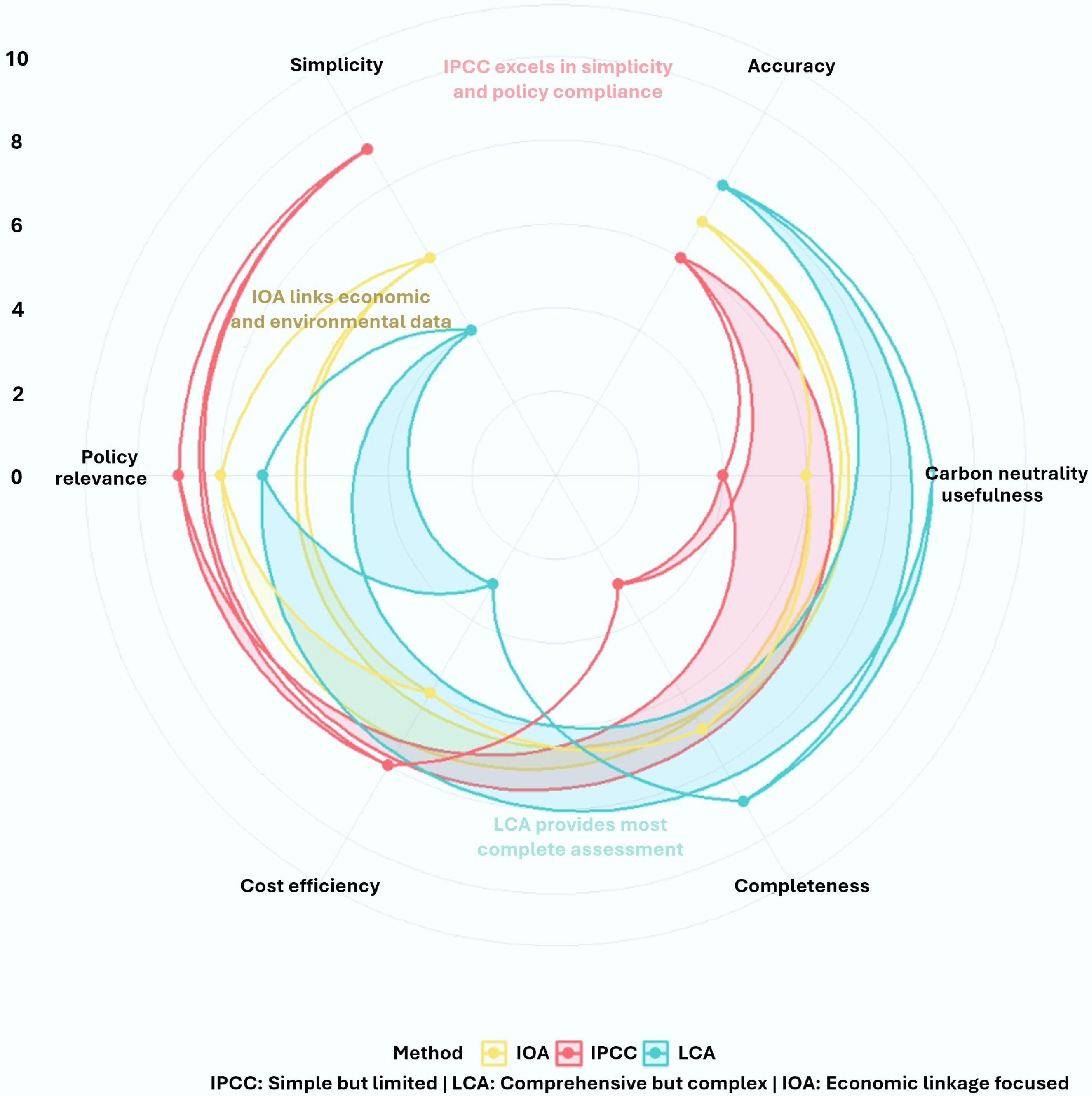
Figure 6.
Comparative evaluation of carbon accounting methodologies for biochar. Radar plot showing relative performance scores (0 = low, 10 = high) across six evaluation criteria. Each method displays characteristic strengths: IPCC for standardized direct emission estimates, LCA for comprehensive lifecycle analysis, and IOA for economic-environmental linkage assessment. The visualization highlights the methodological trade-offs necessary for selecting appropriate carbon assessment approaches in biochar research and policy development.
-
Pyrolysis temperature Specific surface
area (m2 g−1)Porosity
(cm3 g−1)H/C atomic
ratioO/C atomic
ratioDominant carbon structure Primary functional groups 250–350 °C (Low) 10–50 0.01–0.05 1.0–1.4 0.4–0.7 Amorphous, aliphatic-C –OH, –COOH, –CH3 400–500 °C (Medium) 100–400 0.05–0.15 0.5–0.8 0.2–0.4 Mixed aliphatic/aromatic Quinones, phenols 600–700 °C (High) 400–800 0.15–0.30 0.3–0.5 0.05–0.15 Condensed aromatic-C Graphitic domains, π-π* > 800 °C (Very high) 800–1,200 0.30–0.50 < 0.3 < 0.05 Highly graphitic, turbostratic Conjugated π-electrons * H/C and O/C ratios are indicative of aromaticity and stability: lower values correspond to higher carbon stability. Data were synthesized from multiple feedstocks including wood, straw, and manure sources[51]. Table 1.
Key physicochemical properties of biochar as a function of pyrolysis temperature
-
Aspect Life cycle assessment (LCA) Input-output analysis (IOA) Hybrid approach (LCA + IOA) System boundary Cradle-to-gate or cradle-to-grave. Includes: (1) Feedstock collection, (2) Transportation, (3) Pyrolysis, (4) Application. Excludes indirect economic effects. Economy-wide. Captures all sectoral interconnections. Includes direct and indirect emissions from all related industries (mining, manufacturing, services). Combines: (1) Process-specific LCA for pyrolysis, (2) IOA for upstream supply chains (steel for reactors, electricity grid). Data requirements Primary process data (e.g., pyrolysis energy use, transportation distances). Secondary data from Ecoinvent/GaBi databases. High resolution but limited scope. National/regional input-output tables (e.g., USEEIO, EXIOBASE). Sectoral monetary flows and emission factors. Broad but aggregated. Integrated dataset: Process inventories + IO tables. Requires data alignment between physical and monetary units. Carbon accounting results (example) Net sequestration: −0.8 to −1.2 t CO2e per t biochar (including: −2.8 t from carbon stability, +0.5 t from production, +0.3 t from transport). Net economy-wide impact: −0.3 to +0.2 t CO2e per t biochar (includes market-mediated effects: fuel substitution, land-use changes, sectoral shifts). Net impact: −0.6 to −0.9 t CO2e per t biochar. Captures both engineering precision and economy-wide ripple effects. Key differences in results Consistently shows negative emissions (−0.5 to −1.5 t CO2e per t). Ignores market effects (e.g., increased fertilizer demand). Sensitive to carbon stability factor (0.7–0.9). Can show positive emissions in some scenarios due to economic rebound effects. Captures sectoral displacement (e.g., reduced coal use). Highly sensitive to regional economic structure. Intermediate results between LCA and IOA extremes. Accounts for key supply chain nodes with precision. Can identify policy leakage (emissions shifting to other sectors). Error ranges and uncertainty ±25%–40%
• Process data variability (e.g., pyrolysis efficiency: ±15%).
• Carbon stability uncertainty (±20%).
• Allocation methods (mass vs energy: ±10%).±50%–100%
• Sector aggregation error (e.g., 'chemical industry' includes diverse processes).
• Price vs physical unit misalignment.
• Temporal lag in IO tables (two to five years).±30%–50%
• Hybridization errors (mismatch between process and IO data).
• Boundary selection bias (which processes get detailed LCA).
• Double-counting risk between LCA and IOA components.Optimal application scenarios Technology comparison (slow vs fast pyrolysis). Project financing (carbon credit verification). Process optimization (identifying emission hotspots). Regional policy planning (subsidy impact assessment). National carbon budgeting (economy-wide decarbonization pathways). Trade analysis (import/export embodied carbon). Strategic decision-making for large-scale deployment. Carbon pricing scheme design. International reporting (UNFCCC, IPCC Tier 3 methods). Limitations Truncation error (omits distant supply chain effects). Static analysis (no market feedback). Data intensive for site-specific studies. Low technological resolution (cannot distinguish pyrolysis types). Homogeneity assumption (all products in a sector are identical). Complex implementation (requires specialized expertise). Computationally intensive. Limited standardized frameworks. Validation methods Sensitivity analysis (Monte Carlo). Peer-reviewed databases (Ecoinvent). Third-party verification (ISO 14044). Cross-regional comparison (comparing different IO tables). Historical data back-testing. Sectoral disaggregation (using make/use tables). Convergence testing (LCA vs IOA results). Scenario analysis (high/low biochar adoption). Expert elicitation (Delphi method). Table 2.
Comparison of life cycle assessment (LCA) and input-output analysis (IOA) methods for carbon accounting in biochar projects
-
Sector Role in biochar system Key IO relationships Environmental link Agriculture Feedstock supplier → Provides biomass residues Sells biomass to biochar sector; Purchases biochar for soil amendment Provides carbon-negative feedstock; Reduces field burning emissions Biochar
productionCore processing → Converts biomass to stable carbon Purchases from multiple sectors; Sells to agriculture/energy/waste Direct pyrolysis emissions; Creates net carbon sink via stable C Energy Energy provider → Powers pyrolysis;
Can use syngas byproductSells electricity to biochar sector; May purchase syngas fuel Energy source emissions offset by renewable syngas utilization Transport Logistics network → Moves feedstock and final product Serves all sectors in supply chain; Major cost component Transport emissions partially offset by reduced fertilizer transport needs Waste
managementFeedstock source → Agricultural/forestry wastes Provides low-cost inputs; Reduces waste disposal needs Avoids landfill CH4 emissions; Converts waste to value Manufacturing Equipment supplier → Pyrolysis reactors, handling systems Capital investments; Technology development Embodied carbon in equipment offset by long-term sequestration Table 3.
Biochar's position in environmental input-output analysis
-
Method Applicable scenarios Key advantages Main limitations Ref. IPCC emission coefficient method Initial screening of biochar systems
Policy-level carbon accounting
Standardized reporting for compliance
Rapid assessment of direct emissions
Comparison across standardized protocolsInternationally recognized standard
Simple calculation procedure
Low data requirements
Consistent and comparable results
Fast implementation time
Well-established for direct emissionsOnly accounts for direct emissions
Cannot capture indirect emissions (transport, manufacturing)
Uses generic emission factors that may not be region-specific
No economic linkages considered
Static assessment without temporal dynamics
May underestimate total carbon footprint[8,132,133] Life cycle assessment (LCA) Comprehensive product carbon footprint
Technology comparison (e.g., different pyrolysis methods)
Sustainability certification
Eco-design optimization
'Cradle-to-grave' system analysisComplete system boundary coverage
Captures direct and indirect emissions
Identifies environmental hotspots
Multi-impact assessment (not just climate)
Supports decision-making for process optimization
Dynamic modeling possibleData-intensive and time-consuming
Subjective system boundary definition
Complex modeling requirements
Allocation issues for co-products
Results sensitive to methodological choices
Regional specificity challenges[122] Input-output analysis (IOA) Regional carbon budgeting
Supply chain analysis
Economic-environmental policy planning
Sectoral emission analysis
Macro-scale carbon footprint assessmentCaptures economic interdependencies
Avoids system boundary truncation
Consistent sectoral data framework
Suitable for policy analysis
Time-series analysis capability
Good for regional/national scalesAggregated sector-level data (lacks product specificity)
Static coefficients (assumes fixed relationships)
Limited micro-scale applicability
Data lag issues
Cannot accurately assess temporal dynamics
Regional data availability constraints[134,135] Table 4.
Comparative analysis of carbon assessment methods for biochar systems
Figures
(6)
Tables
(4)