-
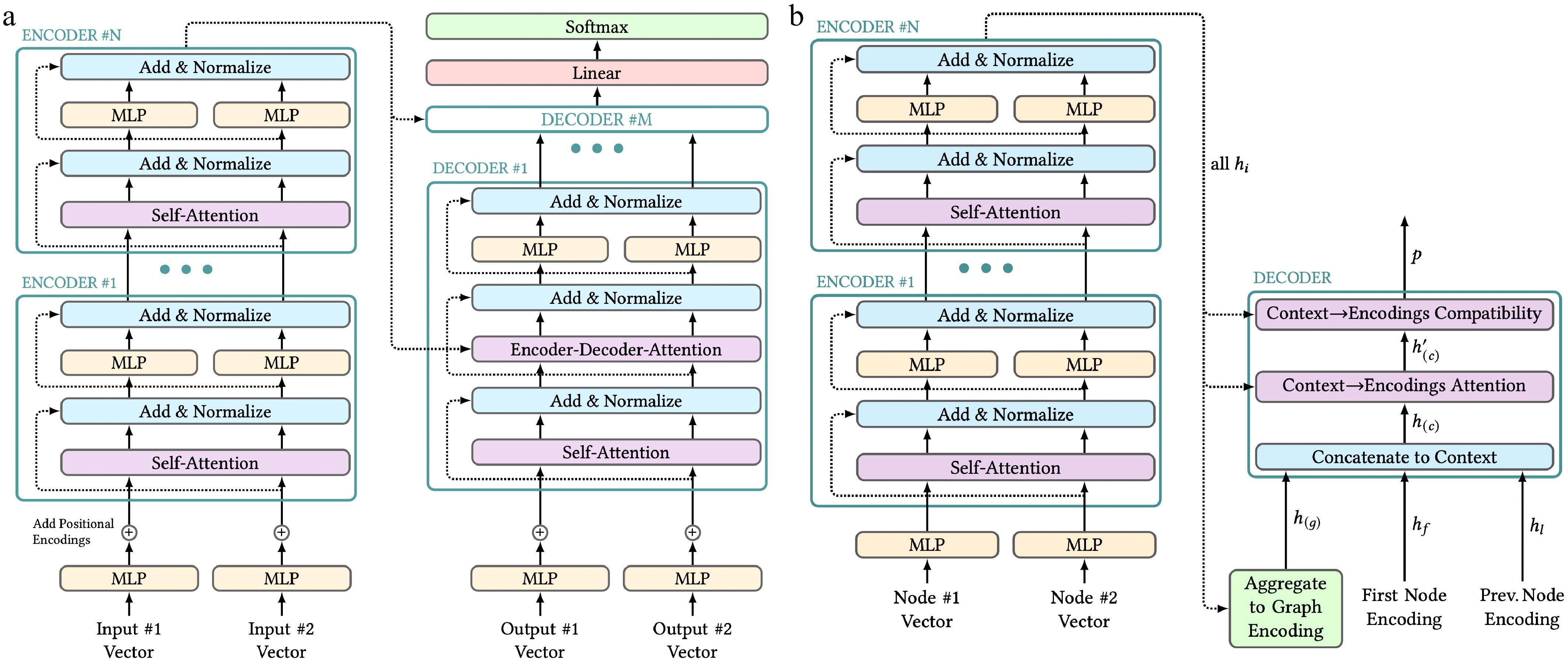
Figure 1.
Transformer architectures. Figure style adapted from Alammar[53]. (a) Structure of a transformer proposed by Vaswani et al.[51] with two representative input vectors on both sides. In practice, any number of inputs can be passed to the encoders and decoders. (b) Structure of Kool, Van Hoof, and Welling's transformer for approximating solutions to the Traveling Salesman Problem.
-
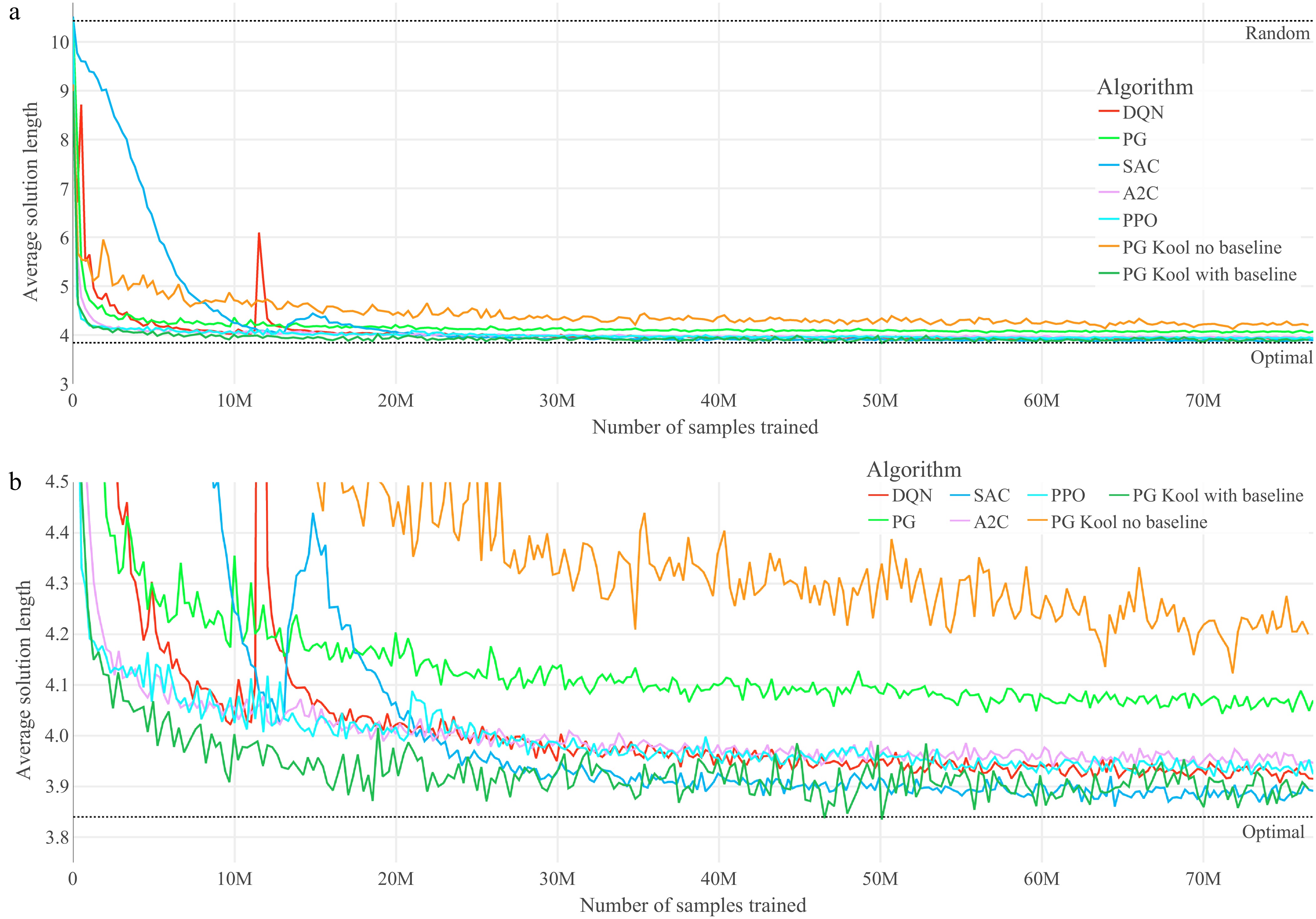
Figure 2.
Training graphs of the optimized agents for the TSP. (a) Performance throughout the training of the seven optimized agents on TSP. (b) Magnified performance throughout the training of the seven optimized agents on TSP.
-
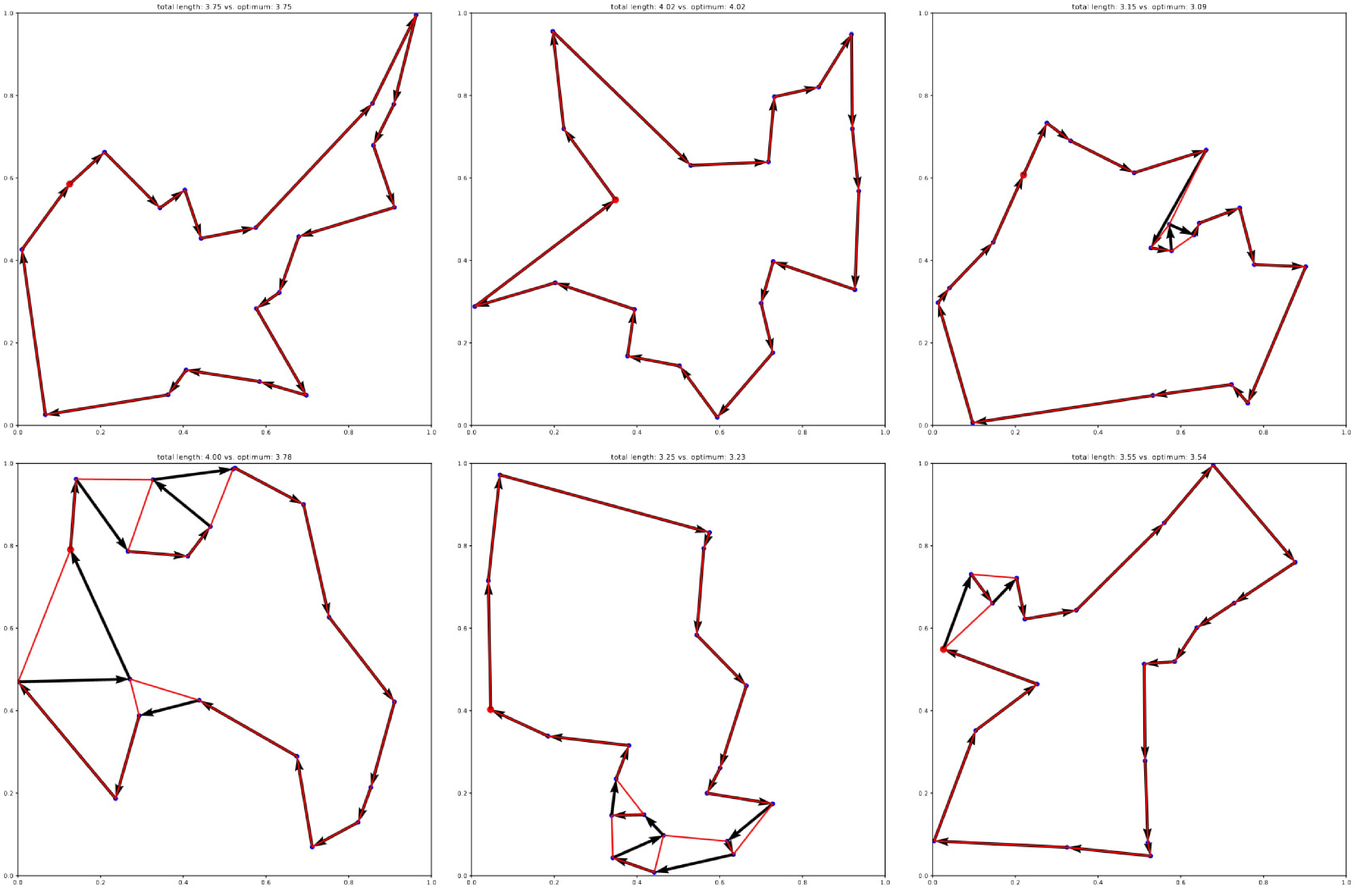
Figure 3.
Exemplary solutions of the best-performing agent (SAC) on the 20-node TSP. Optimal solutions obtained with Gurobi are overlaid in red.
-
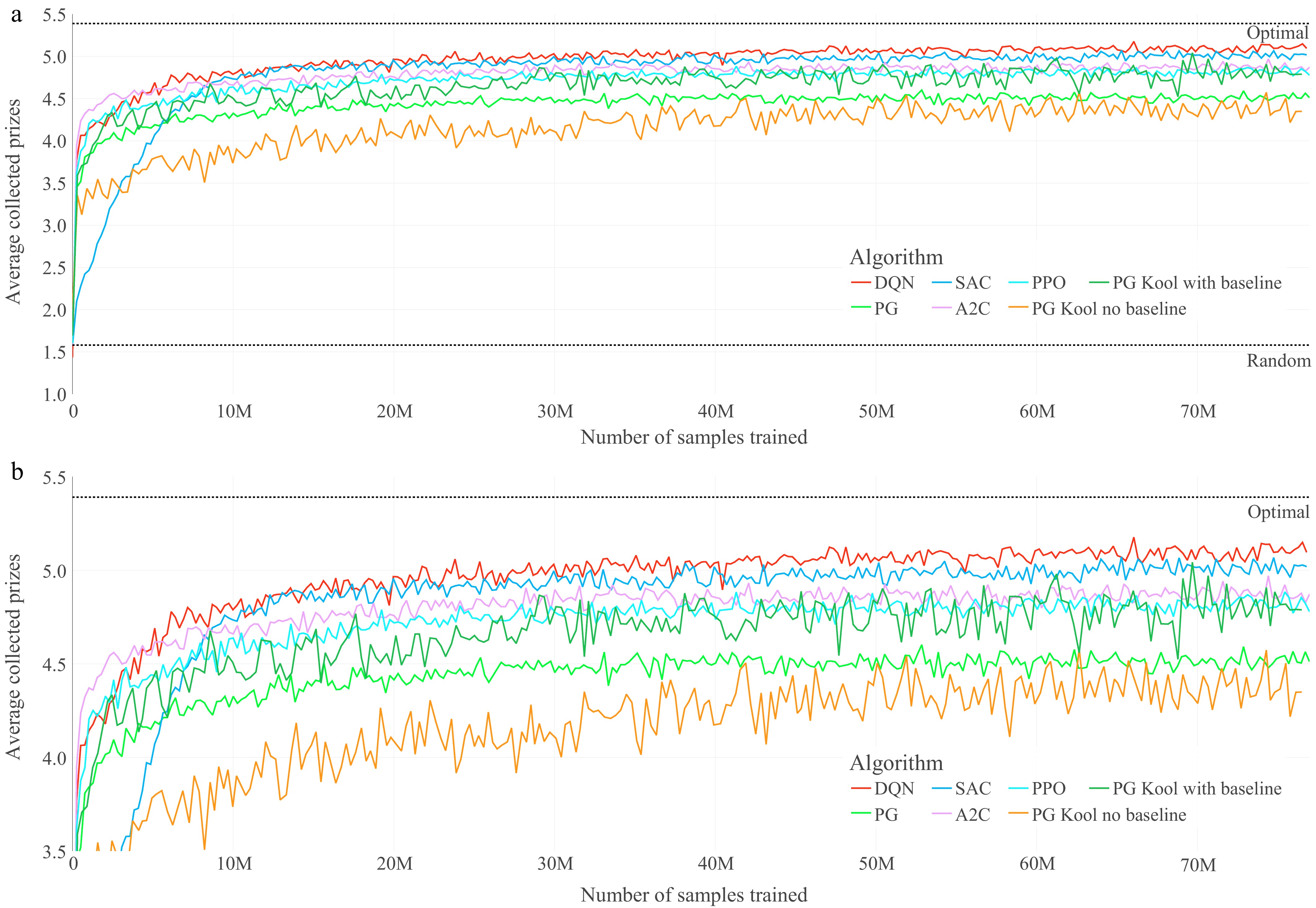
Figure 4.
Training graphs of the optimized agents for the OP. (a) Performance throughout the training of the seven optimized agents on the OP. (b) Magnified performance throughout the training of the seven optimized agents on OP
-
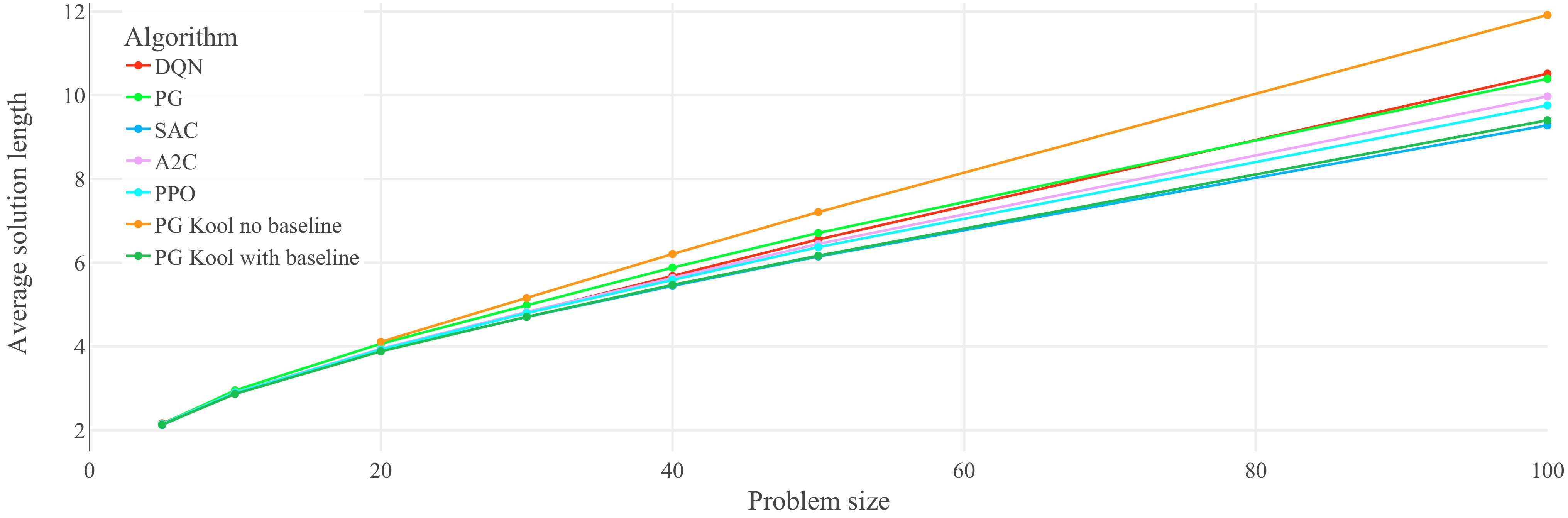
Figure 5.
Performance on untrained problem sizes of the seven optimized agents on the TSP: generalization results for the TSP (lower is better). Each data point represents the average solution length of 1,000 evaluation problem instances. Lines between data points do not represent actual performance but are included for easier identification of trends. Refer to Table 1 for optimal and random solution lengths. The corresponding lines are not included in the plot in order to show the agents' performances on narrower axis scale.
-
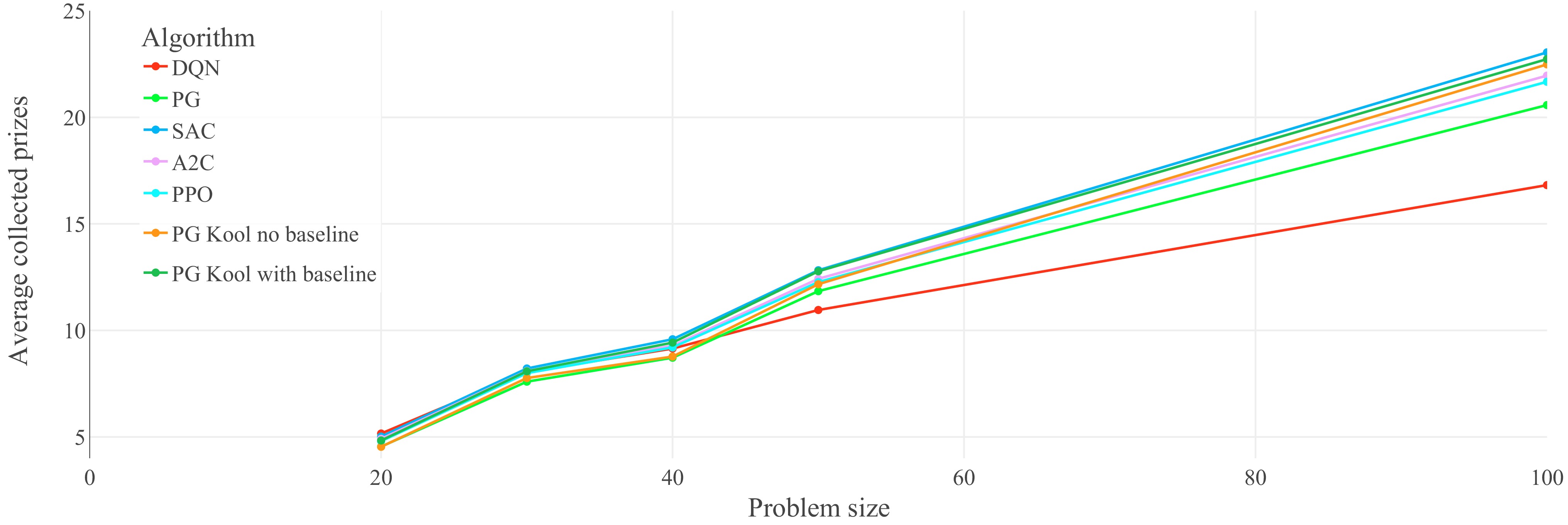
Figure 6.
Performance on untrained problem sizes of the seven optimized agents on the OP: generalization results on the OP (higher is better). Each data point represents the average collected prizes of 1,000 evaluation problem instances. Lines between data points do not represent actual performance but are included for easier identification of trends.
-
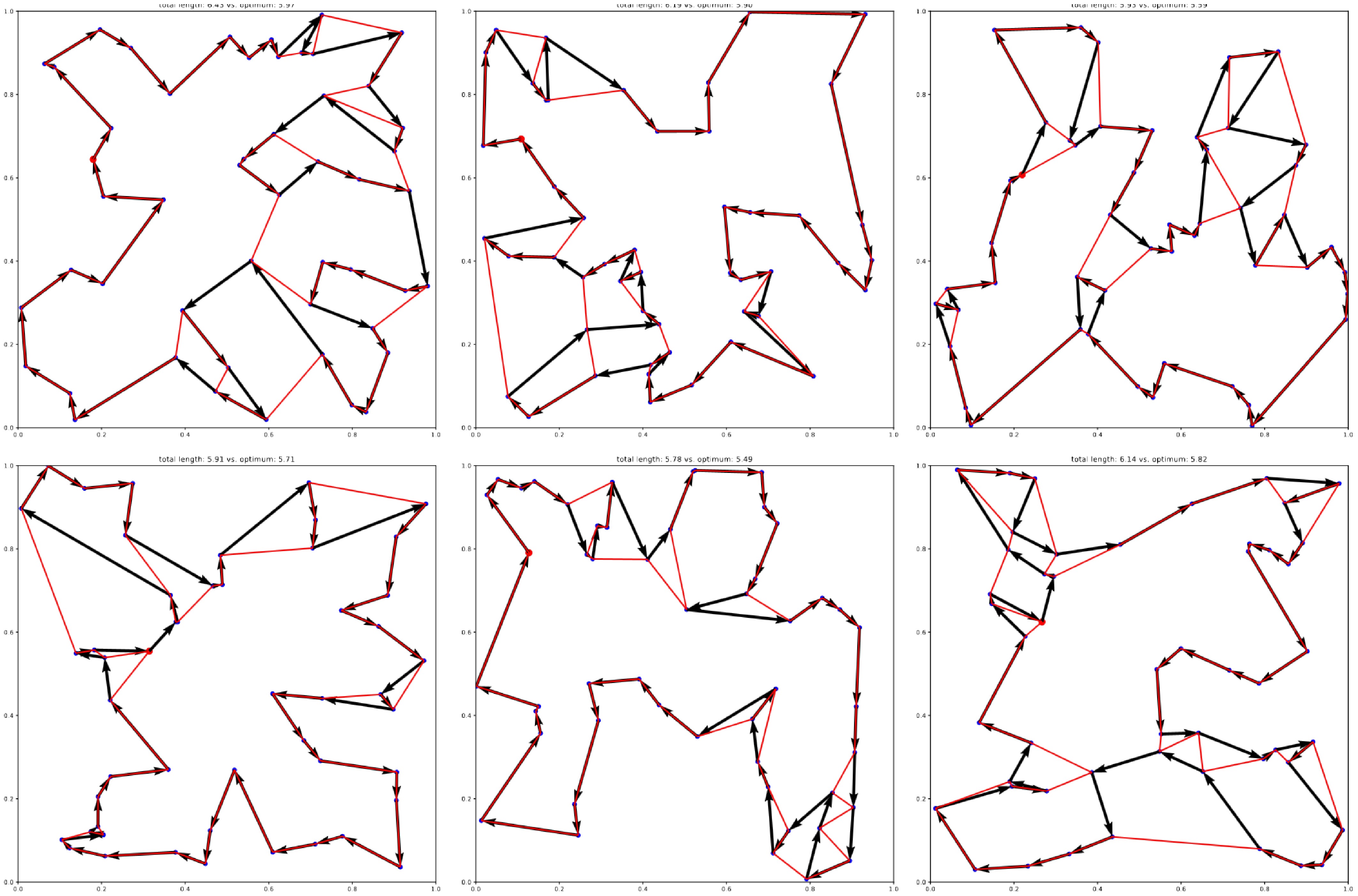
Figure 7.
Exemplary generalization results of the best-performing agent (SAC) trained on the 20-node TSP, and evaluated on 50-node TSP instances. Optimal solutions obtained with Gurobi are overlaid in red.
-
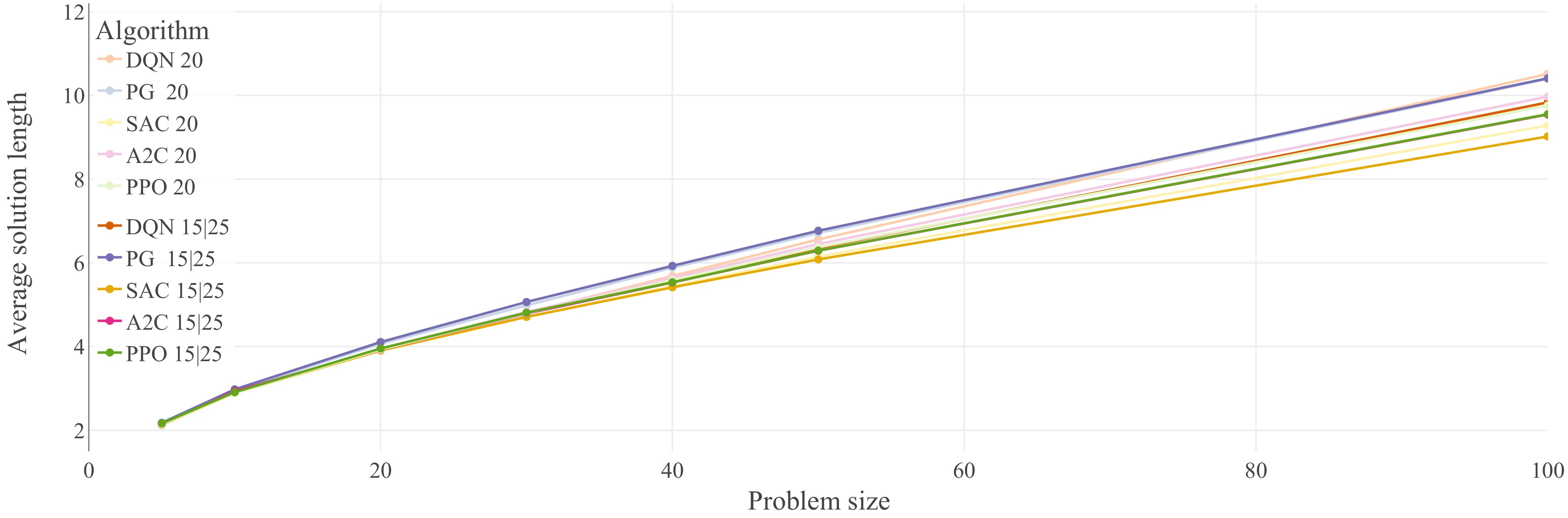
Figure 8.
Performance comparison of five of the optimized agents from Fig. 5 (20-node problems), against the exact same agents trained on 15-node, and 25-node problems. Agents trained on 20-node problems have been assigned the lighter colors, while the agents trained on multiple problem sizes were assigned darker versions of the same colors. Generalization results for the TSP (lower is better). Each data point represents the average solution length of 1,000 evaluation problem instances. Lines between data points do not represent actual performance but are included for easier identification of trends
-
Approach n = 20 n = 50 n = 100 Gap Len Time Gap Len Time Gap Len Time Gurobi (LP, optimal) 0.00% 3.84 7 s 0.00% 5.70 2 m 0.00% 7.76 17 m Bello et al. (greedy) 1.30% 3.89 − 4.39% 5.95 − 6.96% 8.30 − Dai et al. 1.30% 3.89 − 5.09% 5.99 − 7.09% 8.31 − Kool et al. (greedy) 0.52% 3.86 0 s 1.75% 5.80 2 s 4.51% 8.11 6 s Random walk 273% 10.48 − 456% 25.99 − 671% 52.06 − Table 1.
TSP performance comparison adapted from Kool et al.[27] displaying optimality gaps (Gap), average solution lengths (Len), and runtimes (Time) of different approximative heuristic approaches against optimal LP solutions using Gurobi (for n = 20, 50, and 100 nodes).
-
Ranking n = 20 n = 50 n = 100 Len Alg Len Alg Len Alg 1 3.898 SAC 20 6.080 SAC 15,25 9.018 SAC 15,25 2 3.905 SAC 15,25 6.149 SAC 20 9.282 SAC 20 3 3.919 DQN 15,25 6.290 A2C 15,25 9.543 A2C 15,25 4 3.923 A2C 15,25 6.293 PPO 15,25 9.551 PPO 15,25 5 3.928 DQN 20 6.353 DQN 15,25 9.759 PPO 20 6 3.928 PPO 20 6.373 PPO 20 9.832 DQN 15,25 7 3.945 A2C 20 6.449 A2C 20 9.972 A2C 20 8 3.953 PPO 15,25 6.557 DQN 20 10.393 PG 20 9 4.066 PG 20 6.712 PG 20 10.408 PG 15,25 10 4.107 PG 15,25 6.767 PG 15,25 10.514 DQN 20 Table 2.
Detailed scores and ranking of the agents (Alg) from Fig. 8 for problem sizes n = 20, 50, and 100; average solution lengths (Len) are based on the evaluation of 1,000 problem instances.
Figures
(8)
Tables
(2)