-
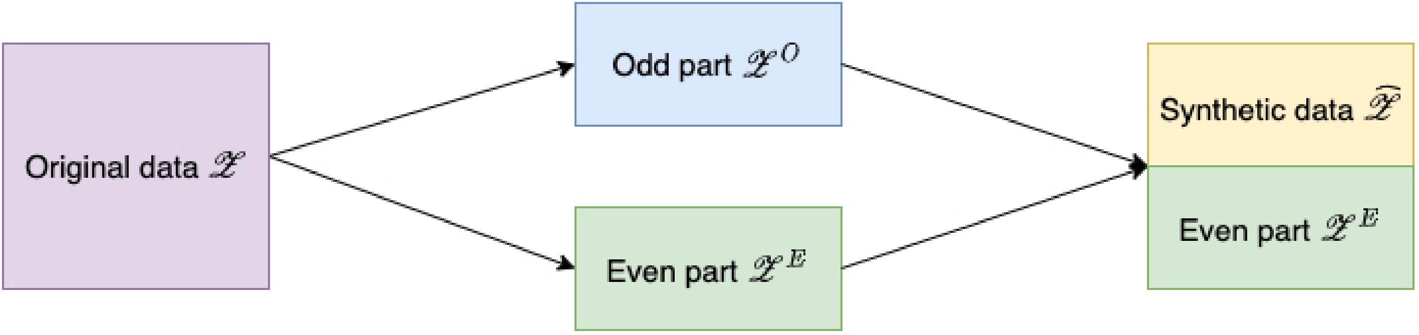
Figure 1.
Flow chart of SD filter.
-
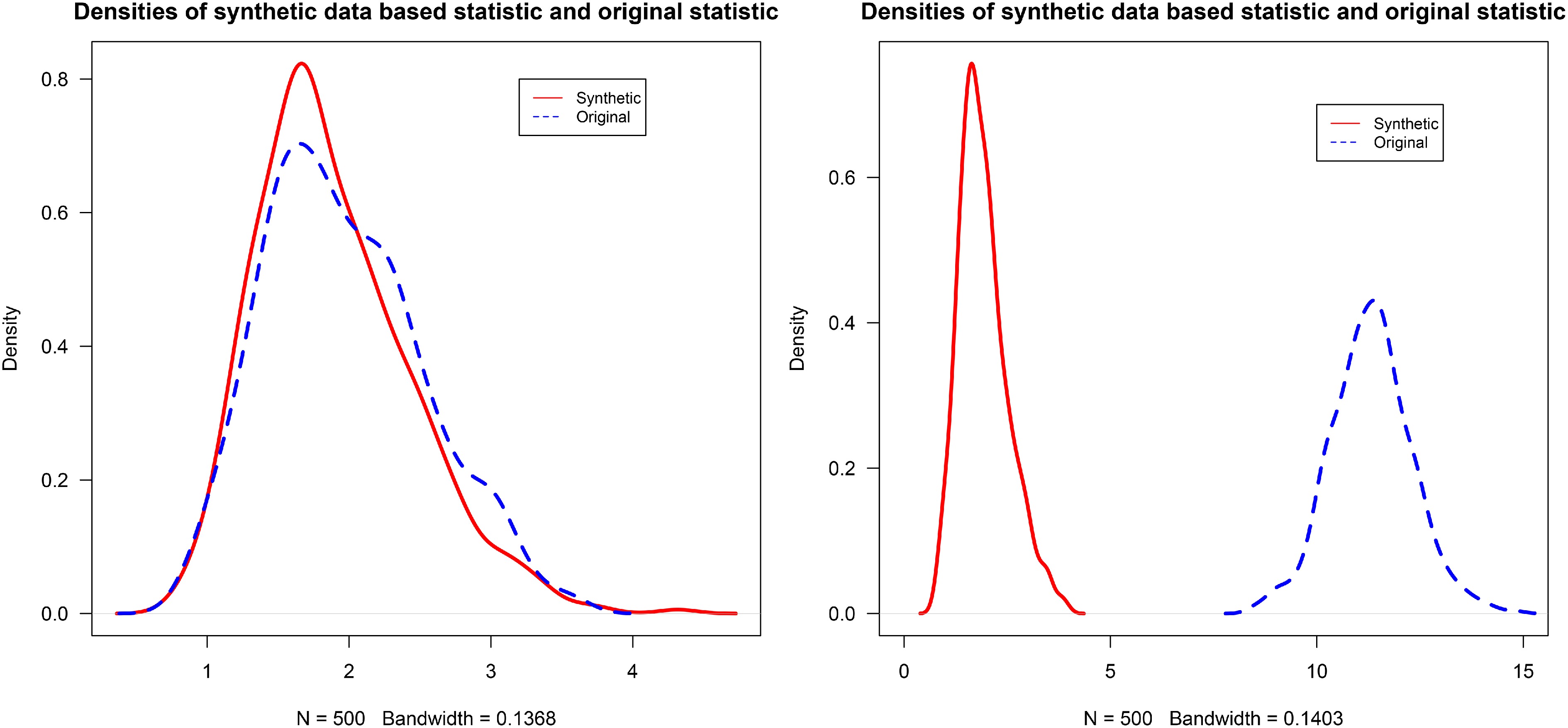
Figure 2.
Densities of the synthetic-data-based statistic and the original statistic under stationary (left) and non-stationary (right) settings. Detailed settings are described in the simulation study.
-
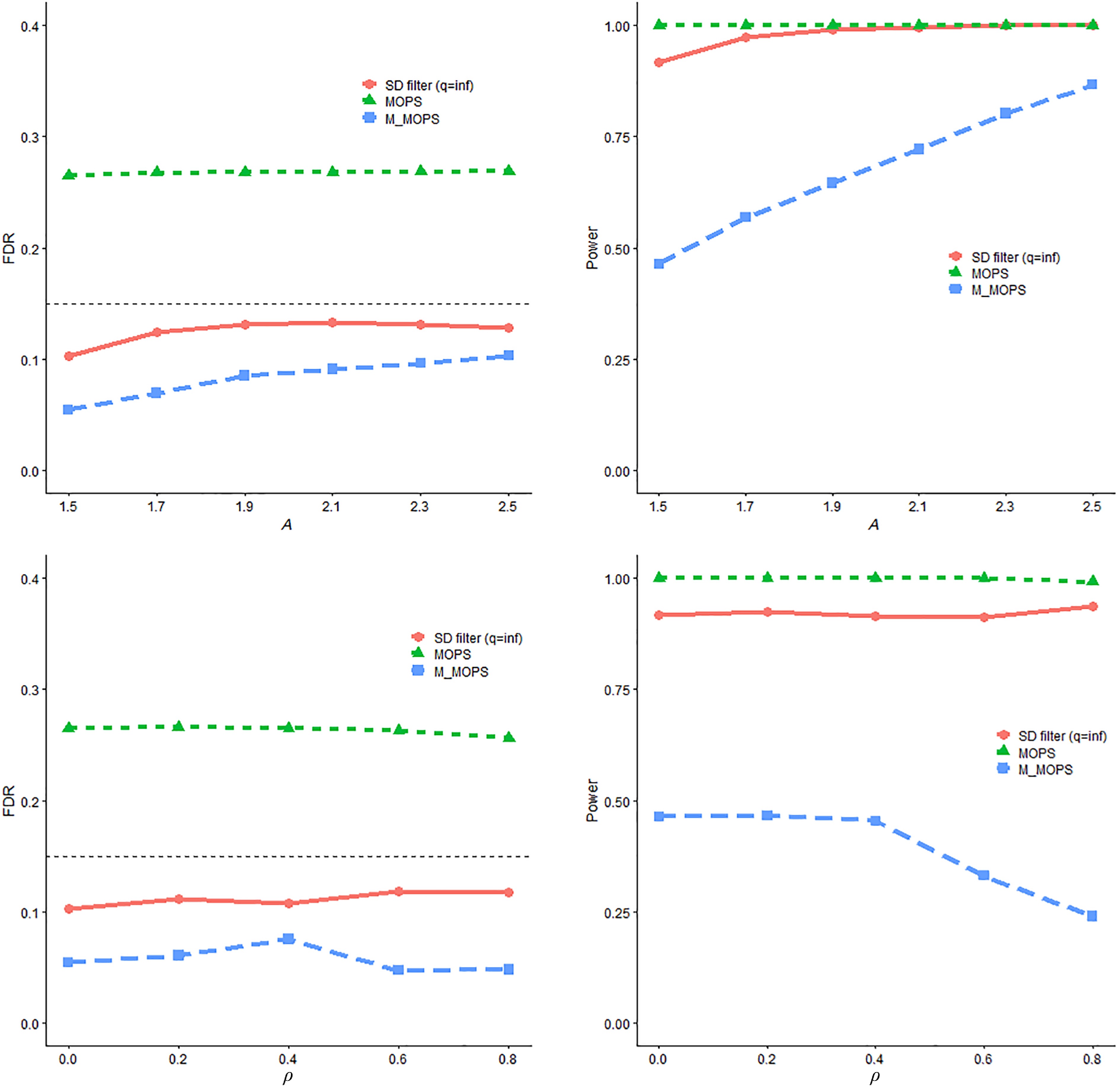
Figure 3.
FDR and power trends with respect to A and
$ \rho $ $ \alpha $ -
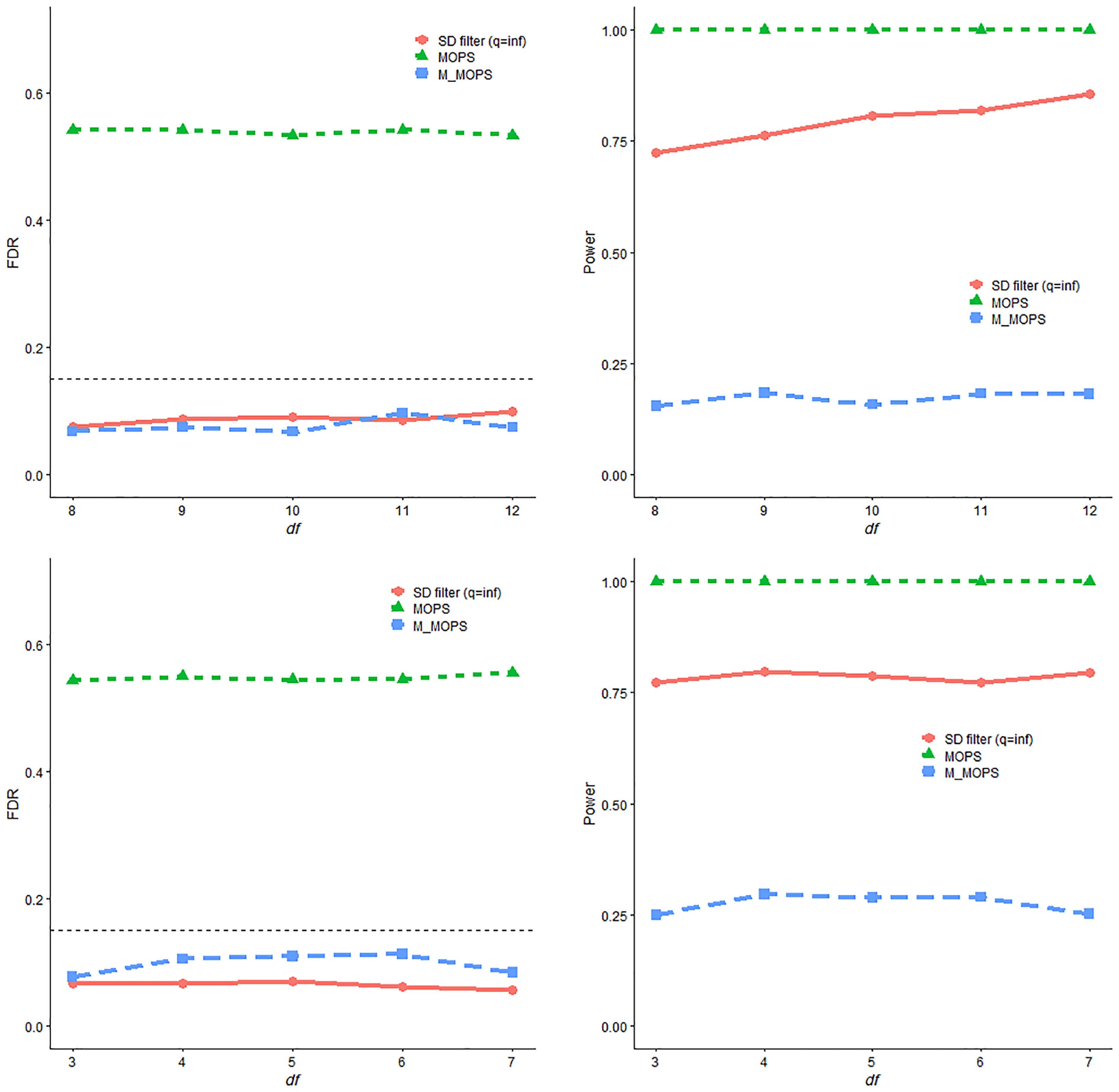
Figure 4.
FDR and power trends with respect to df of the t-distribution and chi-square distribution for SD filter, MOPS, and M-MOPS under the mean change model, where n = 4,000, d = 50,
$ \alpha $ -
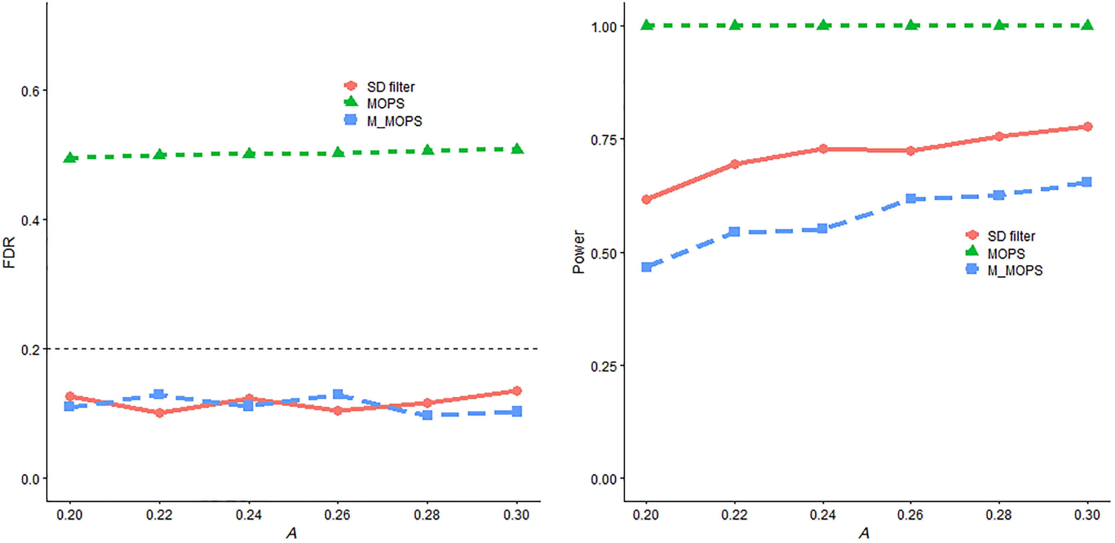
Figure 5.
FDR and power trends with respect to A for SD filter, MOPS, and M-MOPS under the structural breaks linear regression model, where n = 8,000, d = 10,
$ \alpha $ -
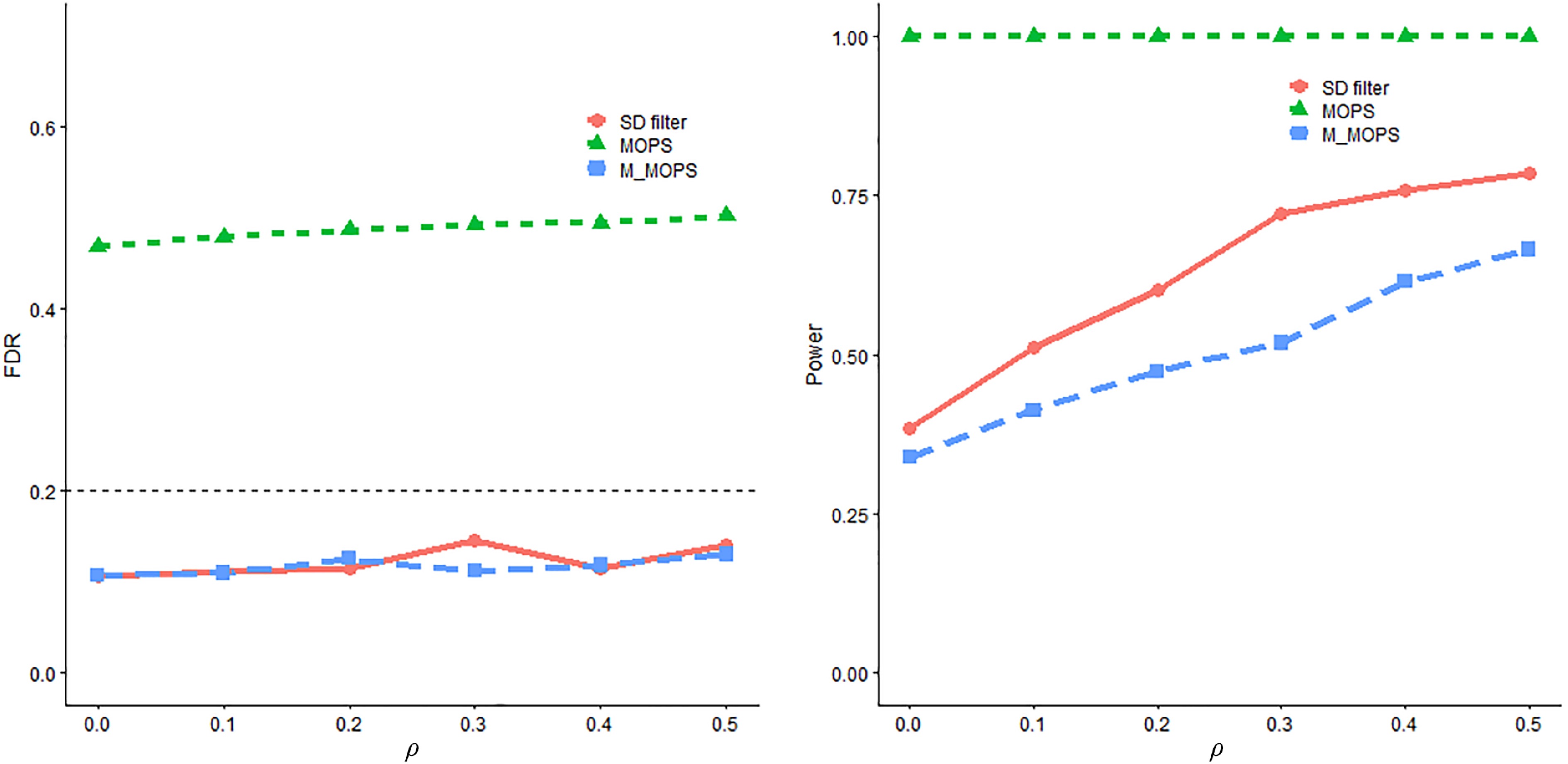
Figure 6.
FDR and power trends with respect to
$ \rho $ $ \alpha $ -
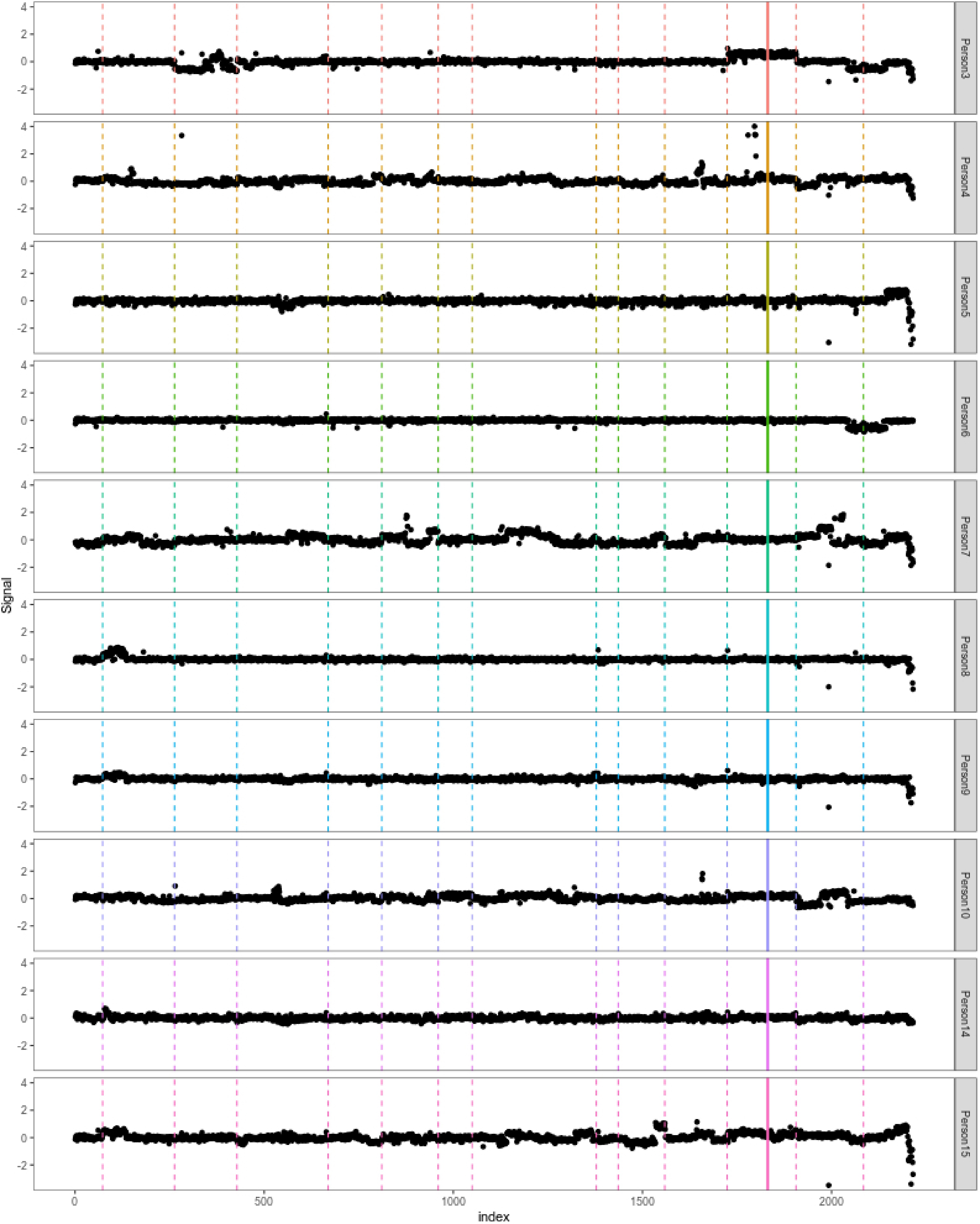
Figure 7.
Detected change-points on bladder tumor micro-array dataset (first ten persons are presented).
-
${\bf Input:}$ $\mathcal Z = \{{\bf{z}}_1, \dots, {\bf{z}}_{2n}\}$ $\alpha$ $\mathcal{A}(\cdot)$ ${\bf Output:}$ $\mathcal T$ 1: Split data into odd and even parts: $ \mathcal{Z}^O = \{ \mathbf{z}_1, \mathbf{z}_3, \dots, \mathbf{z}_{2n-1}\}, \,\, \mathcal{Z}^E = \{ \mathbf{z}_2, \mathbf{z}_4, \dots, \mathbf{z}_{2n}\} $ 2: Detect candidate change-points $ \hat{ \mathcal{S}}=\{ \hat{\tau}_1, $ $\dots, {\hat{\tau}_{\hat{K}_n}}\}$ $ {\mathcal{A}}({\mathcal{Z}}^O) $ 3: for $ k \in 1,\cdots,\hat{K}_n $ 4: Define $ G_k := \left[\lceil(\hat{\tau}_{k-1}+ \hat{\tau}_k)/2\rceil, \lceil(\hat{\tau}_{k} + \hat{\tau}_{k+1})/2\rceil\right) $ $ \hat{\tau}_0 = 0 $ $ \hat{\tau}_{ \hat{K}_n} = 2n $ $ \mathcal{Z}_{G_k}^O := \{ \mathbf{z}_{2i-1}: i \in G_k\} $ $ \mathcal{Z}_{G_k}^E := \{ \mathbf{z}_{2i}: i \in G_k\} $ 5: Compute score function $ \mathbf{s}_i^E $ $ \mathbf{c}_{k}(s)=\sqrt{\dfrac{s(n_k-s)}{n_k}}\left(\dfrac{1}{s} \sum_{i \leqslant s, i \in G_k} \mathbf{s}^E_{i}-\dfrac{1}{n_k-s} \sum_{i \gt s, i \in G_k} \mathbf{s}^E_{i}\right) $ 6: Generate synthetic data $ \tilde{ \mathcal{Z}}_{G_k} $ $ \left\{\xi_{i}\left(\mathbf{s}^O_{i}-\bar{ \mathbf{s}}_k^{O,-}(s) \right), i \leqslant s, i \in G_k \right\} \text{ and } \left\{\xi_{i}\left(\mathbf{s}^O_{i}-\bar{ \mathbf{s}}_k^{O,+}(s) \right), i \gt s, i \in G_k \right\} $ $ \xi_i \sim N(0,1) $ 7: Compute synthetic CUSUM $ \tilde{ \mathbf{c}}_{k}(s)=\sqrt{\dfrac{s(n_k-s)}{n_k}}\left(\dfrac{1}{s} \sum_{i \leqslant s, i \in G_k} \xi_{i}\left(\mathbf{s}^O_{i}-\bar{ \mathbf{s}}_k^{O,-}(s) \right)- \dfrac{1}{n_k - s}\sum_{i \gt s, i \in G_k} \xi_{i}\left(\mathbf{s}^O_{k}-\bar{ \mathbf{s}}_k^{O,+}(s) \right) \right) $ 8: Calculate: $ T_k^q = \max_{s \in G_k^*} \| \mathbf{c}_k(s)\|_q, \,\, \tilde{T}_k^q = \max_{s \in G_k^*} \|\tilde{ \mathbf{c}}_k(s)\|_q $ $ W_k^{side,q} = (T_k^q - \tilde{T}_k^q) \cdot T_k^q(\mathcal{Z}_{G_k}^O) $ 9: end for 10: Obtain threshold $ T(\alpha) $ $ T(\alpha) = \min \left\{ t : \dfrac{1 + \#\{k: W_k^{side,q} \leqslant -t\}}{\#\{k: W_k^{side,q} \geqslant t\} \vee 1} \leqslant \alpha \right\} $ 11: Select final change-point set: $ \mathcal{T}^{side} = \{\hat{\tau}_k \in \hat{ \mathcal{S}} : W_k^{side,q} \geqslant T(\alpha)\} $ 12: return $ \mathcal{T}^{side} $ Table 1.
Synthetic data filter (SD filter) for MCP detection.
Figures
(7)
Tables
(1)