Back Article

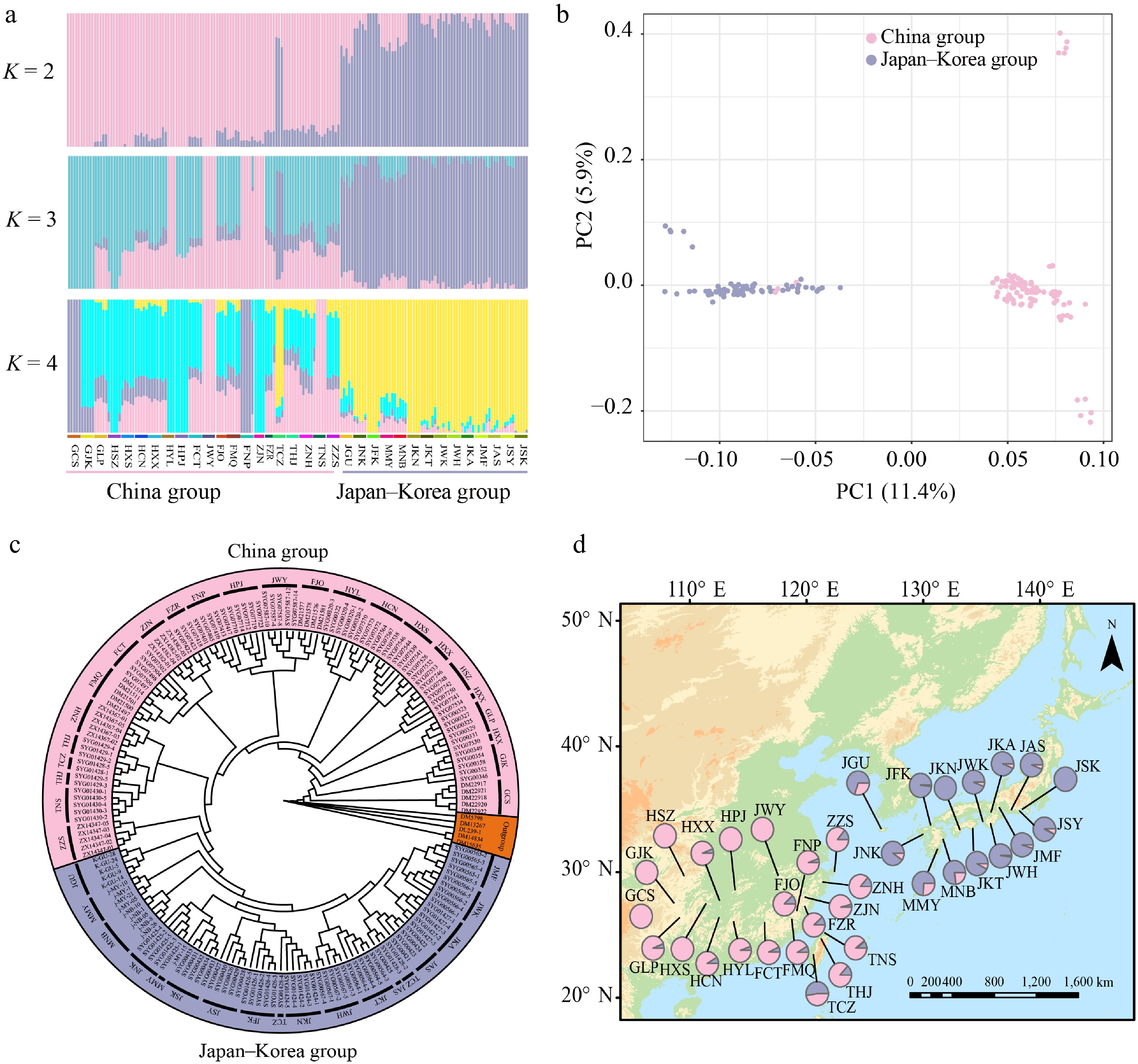
Figure 1. 

Geographic distribution and population genetic structure of Quercus gilva. (a) ADMIXTURE bar plots for K = 2, K = 3, and K = 4. The x-axis represents populations, and the y-axis shows the inferred ancestry proportions. (b) Principal component analysis (PCA) with color-coding to indicate different groups of Q. gilva. Light pink and lavender-blue represent clusters in China, and Japan–Korea, respectively. (c) Maximum likelihood (ML) phylogenetic tree of 171 Q. gilva individuals and five outgroup taxa. (d) Geographical distribution of the 35 sampled populations with color-coded groupings based on the structure analysis (K = 2).

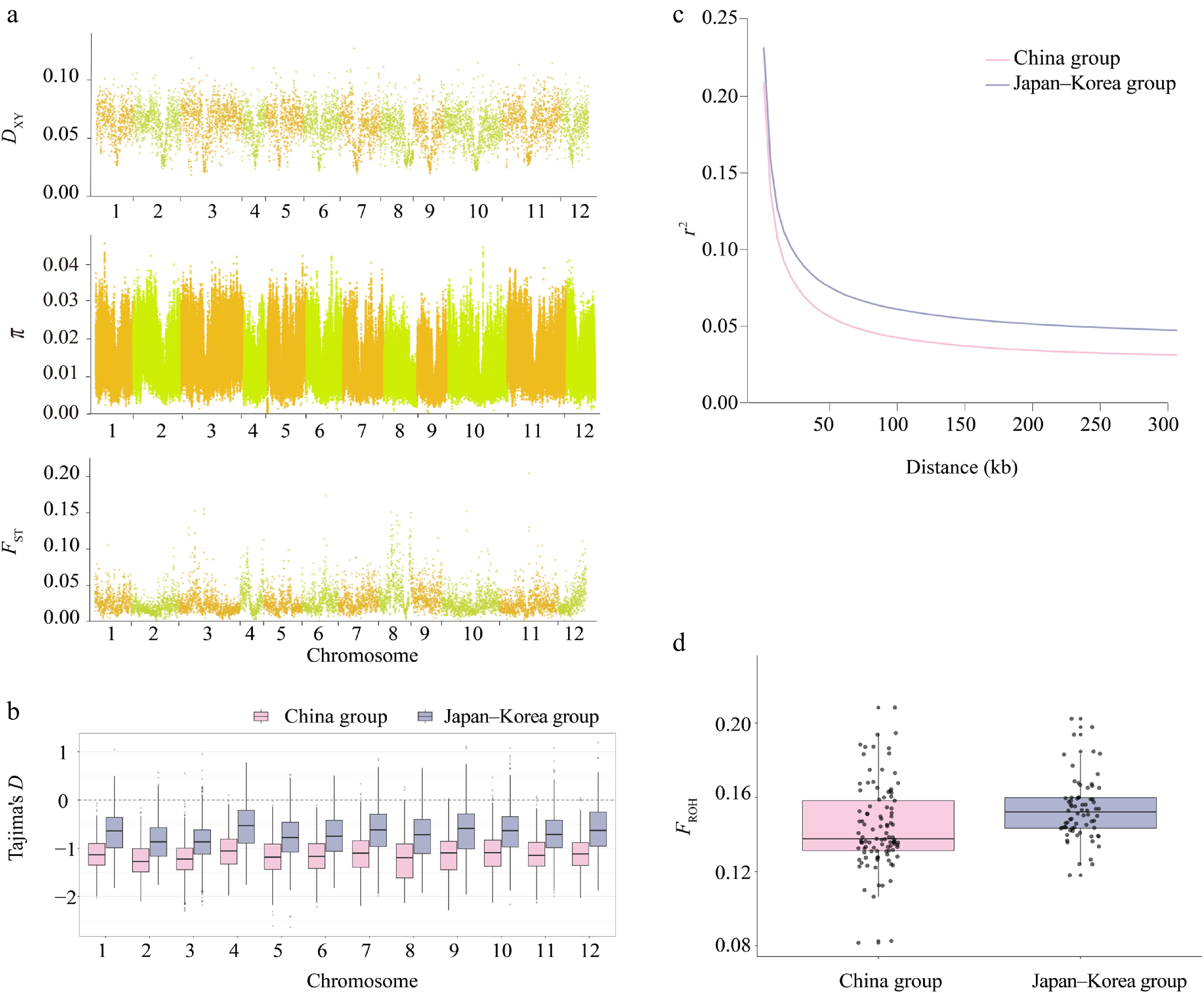
Figure 2. 

Heterogeneity in genomic diversity and genomic divergence between the China and Japan–Korea groups of Q. gilva. (a) Manhattan plot showing the distribution of D_XY, π, and F_ST values between the two populations across chromosomes 1–12. The x-axis indicates the chromosomal position (cumulative physical position), and the y-axis indicates the values of D_XY, π, and F_ST. Each data point corresponds to a 100-kb sliding window. Chromosomes are alternately colored in light orange and light green to distinguish chromosome boundaries. (b) Comparison of Tajima's D across autosomes between two East Asian clusters. Boxplots show the distribution of Tajima's D values on chromosomes 1–12 for the China group (light pink) and the Japan–Korea group (lavender blue). (c) Linkage disequilibrium (LD) decay patterns in the two groups. (d) Comparison of inbreeding coefficients (F_ROH) between two populations of Q. gilva. Light pink and lavender blue represent the China group and the Japan–Korea group, respectively.

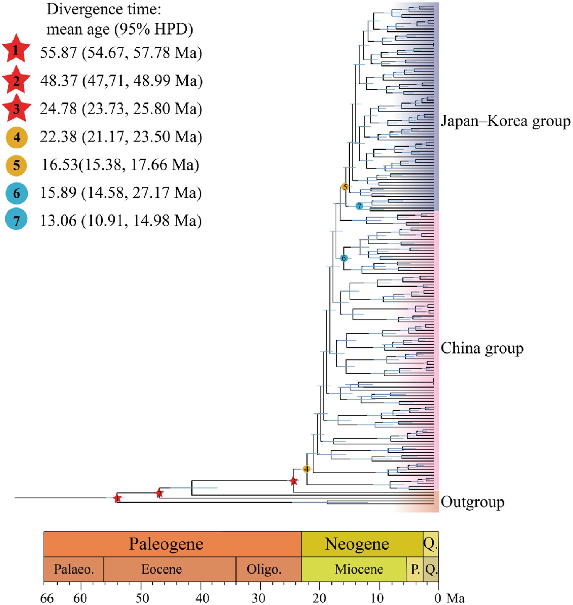
Figure 3. 

Divergence times estimated using BEAST, with blue bars indicating 95% highest posterior density (HPD) intervals. Note that red five-pointed stars indicate the three selected fossil calibrations. Geological time abbreviation: P. = Pliocene; Q. = Quaternary. Circles represent divergence time estimates for Q. gilva populations: (4) divergence of Q. gilva populations in China; (5) divergence between the China and Japan–Korea groups; (6) divergence between the Zhejiang and Taiwan populations; (7) divergence between Japanese and Korean populations.

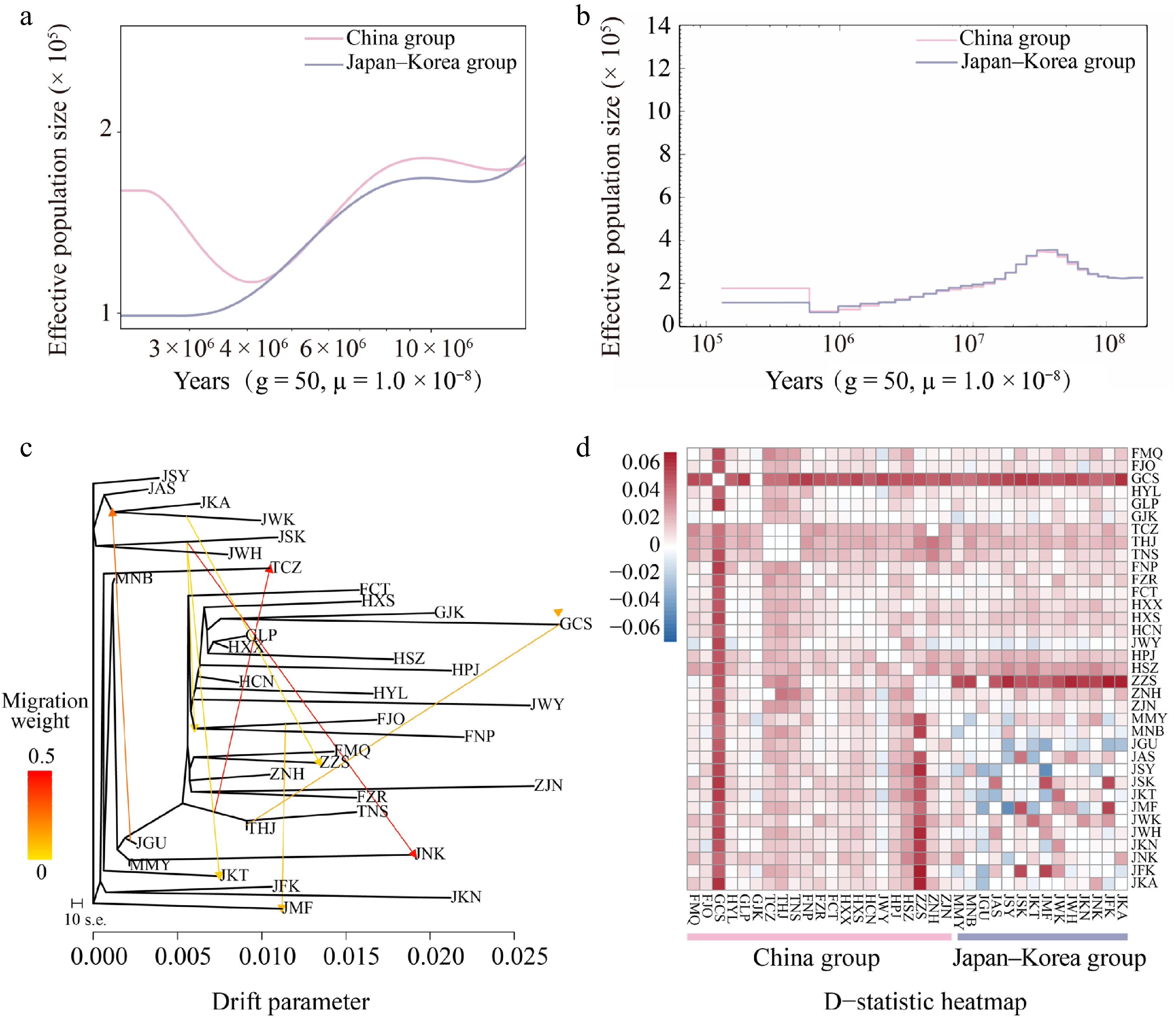
Figure 4. 

Inferred demographic histories of the China (light pink) and Japan–Korea groups (lavender-blue) based on (a) SMC++, and (b) PSMC analyses. (c) Maximum likelihood (ML) tree constructed with TreeMix, allowing for eight migration events. Migration arrows are color-scaled by weight. (d) Introgression analysis with Dsuite was presented as a heatmap, where darker shades indicate higher introgression proportions between populations. For each trio (P1, P2, P3), the D value was mapped to P2 vs. P3 as positive (+D) and to P1 vs. P3 as negative (–D).

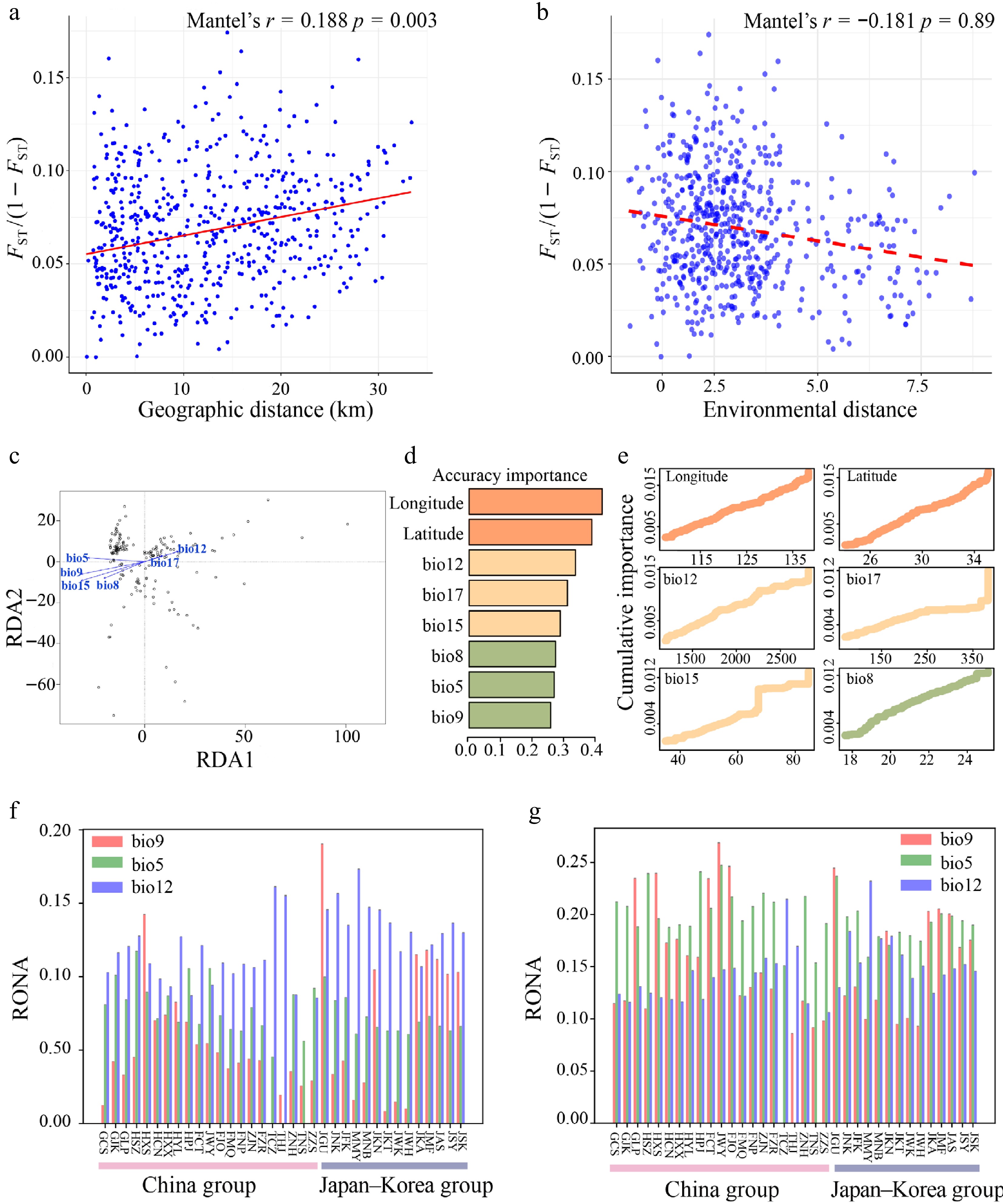
Figure 5. 

(a) Mantel test of genetic distance [F_ST/(1 − F_ST)] vs. geographical distance. (b) Mantel test of genetic distance [F_ST/(1 − F_ST)] vs. environmental distance. (c) Redundancy Analysis (RDA) of Q. gilva (Note that the vector length represents the contribution of each environmental variable to the explained variance, while the angles between arrows indicate correlations among variables). (d) Ranked environmental variable importance plot for Q. gilva based on Gradient Forest (GF) analysis. (e) I-spline curves illustrating genetic composition variation along environmental gradients. (f) Key environmental factors influencing Q. gilva vulnerability under SSP126 (2081−2100). (g) Key environmental factors influencing Q. gilva vulnerability under SSP585 (2081–2100).

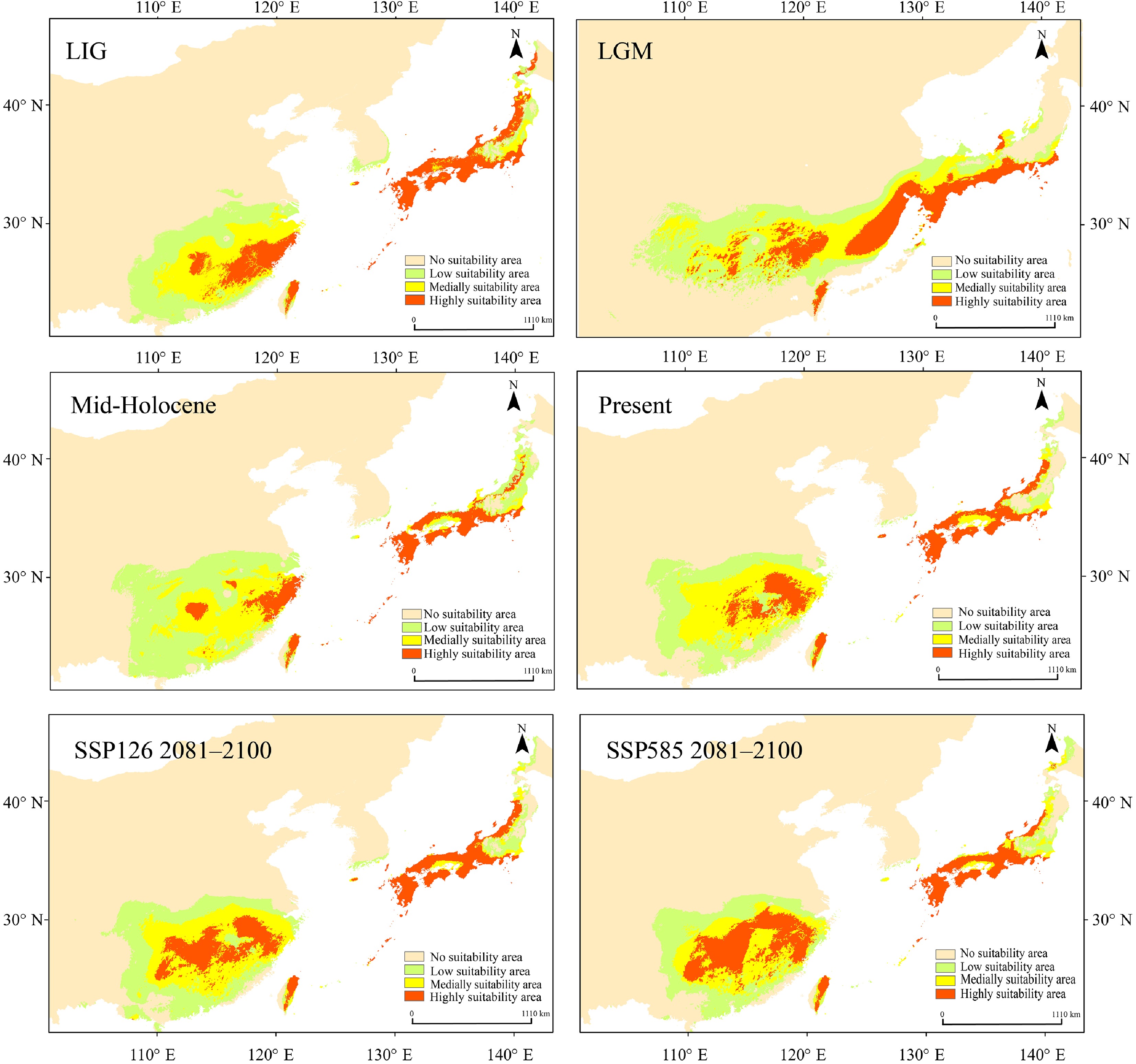
Figure 6. 

Maxent was used to simulate the ecological niches of Q. gilva over six time periods: Last Interglacial (LIG), Last Glacial Maximum (LGM), Mid-Holocene, present, SSP126 2081–2100, and SSP585 2081–2100. Note that the color gradient from light orange to red in the potential distribution areas represents habitat suitability levels for Q. gilva, ranging from unsuitable to optimal conditions.

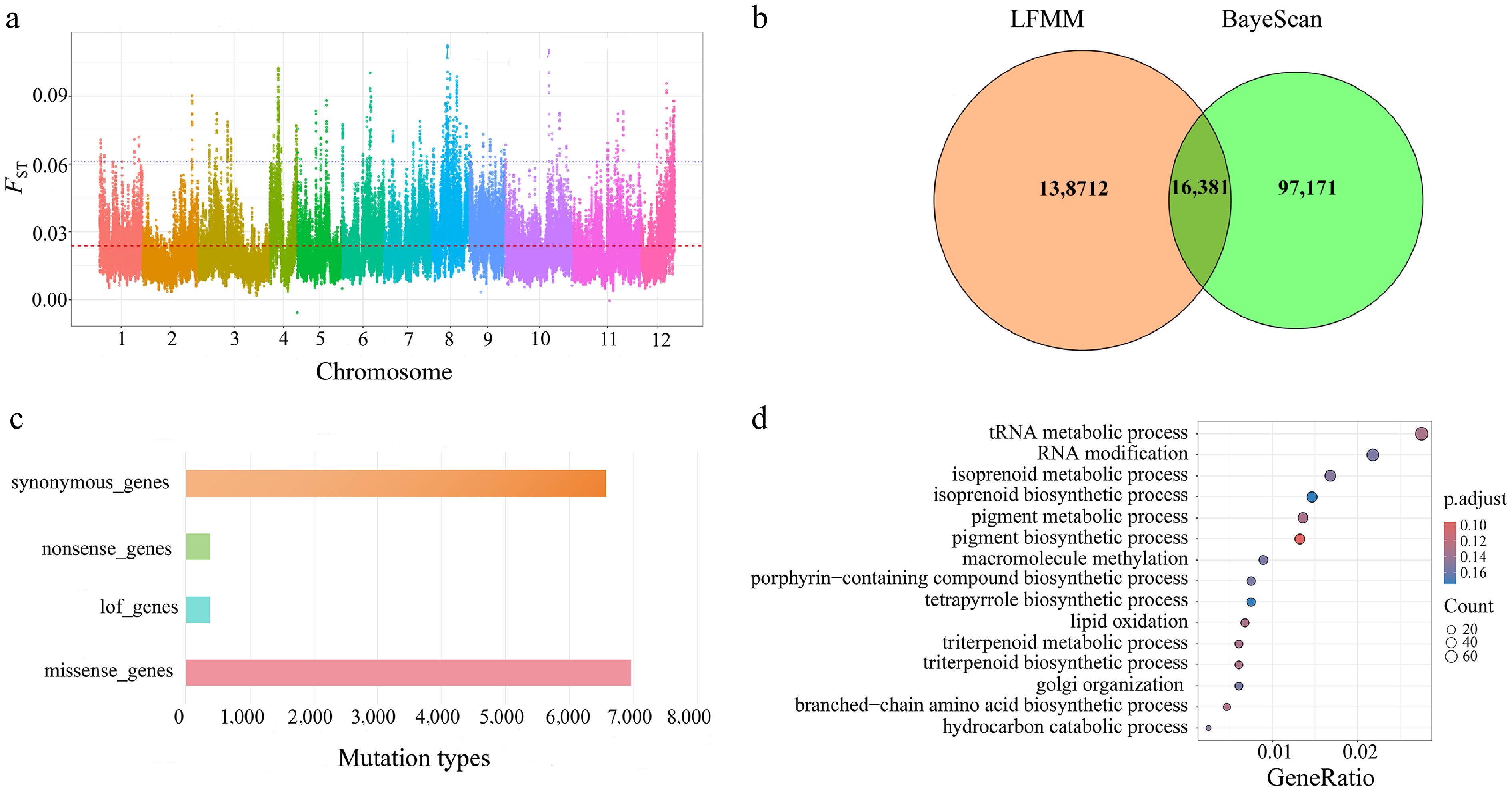
Figure 7. 

(a) Highly polymorphic loci for assessing genetic differentiation. (b) Illustrates a Venn diagram showing the detection of outlier loci based on BayeScan and LFMM. (c) Functional annotation performed using snpEff. (d) The results of GO enrichment analysis for missense mutations.