-
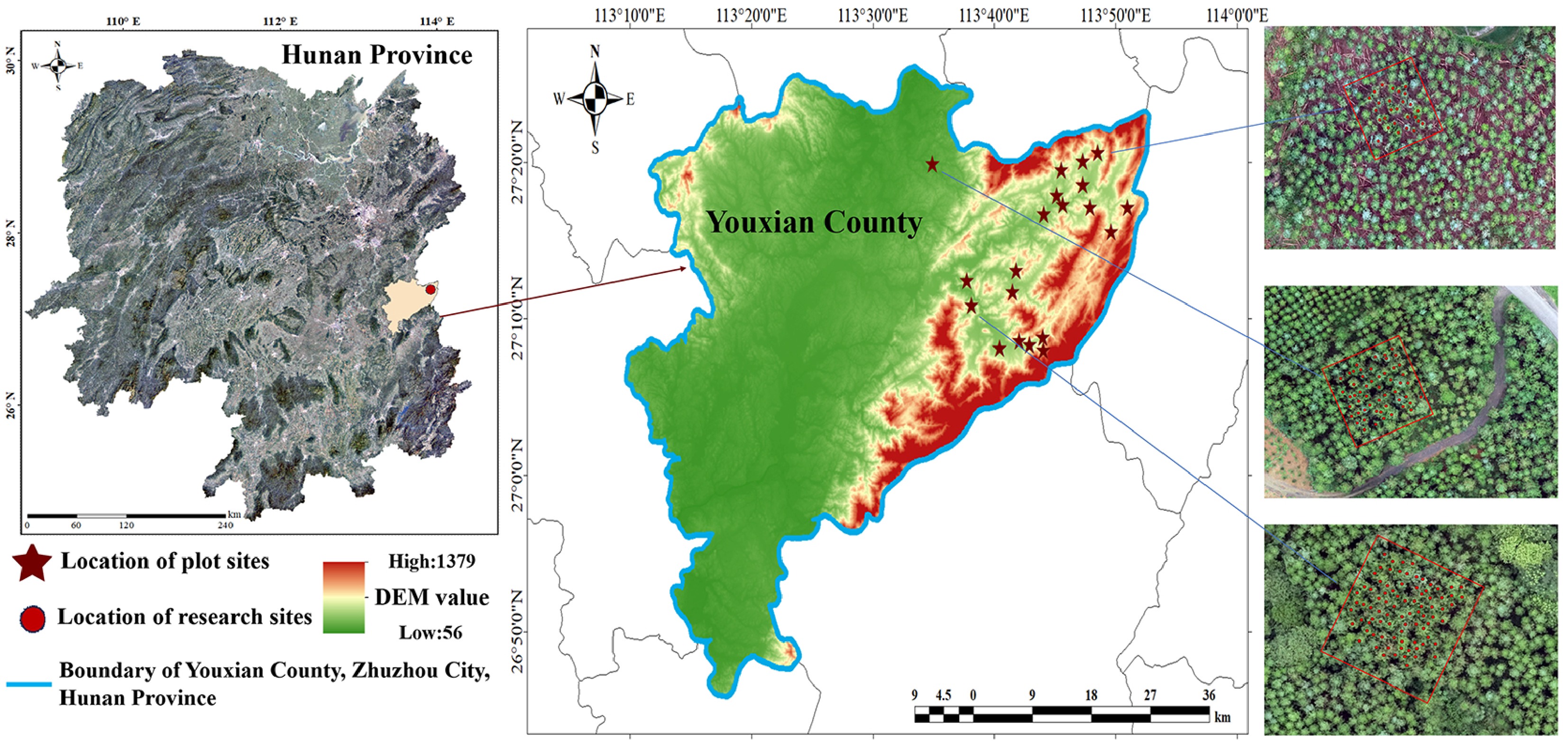
Figure 1.
Distribution of the study area and plot locations. Drawing Review Number: GS(2019)1822.
-
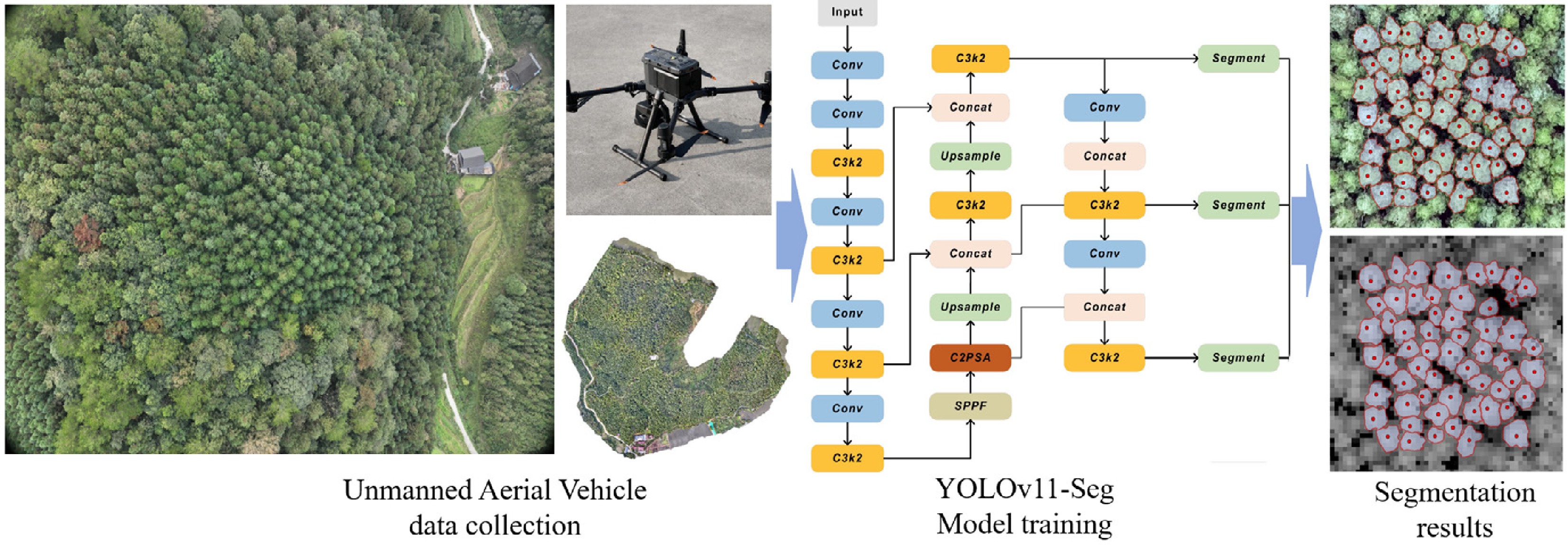
Figure 2.
Data collection and single tree crown segmentation.
-
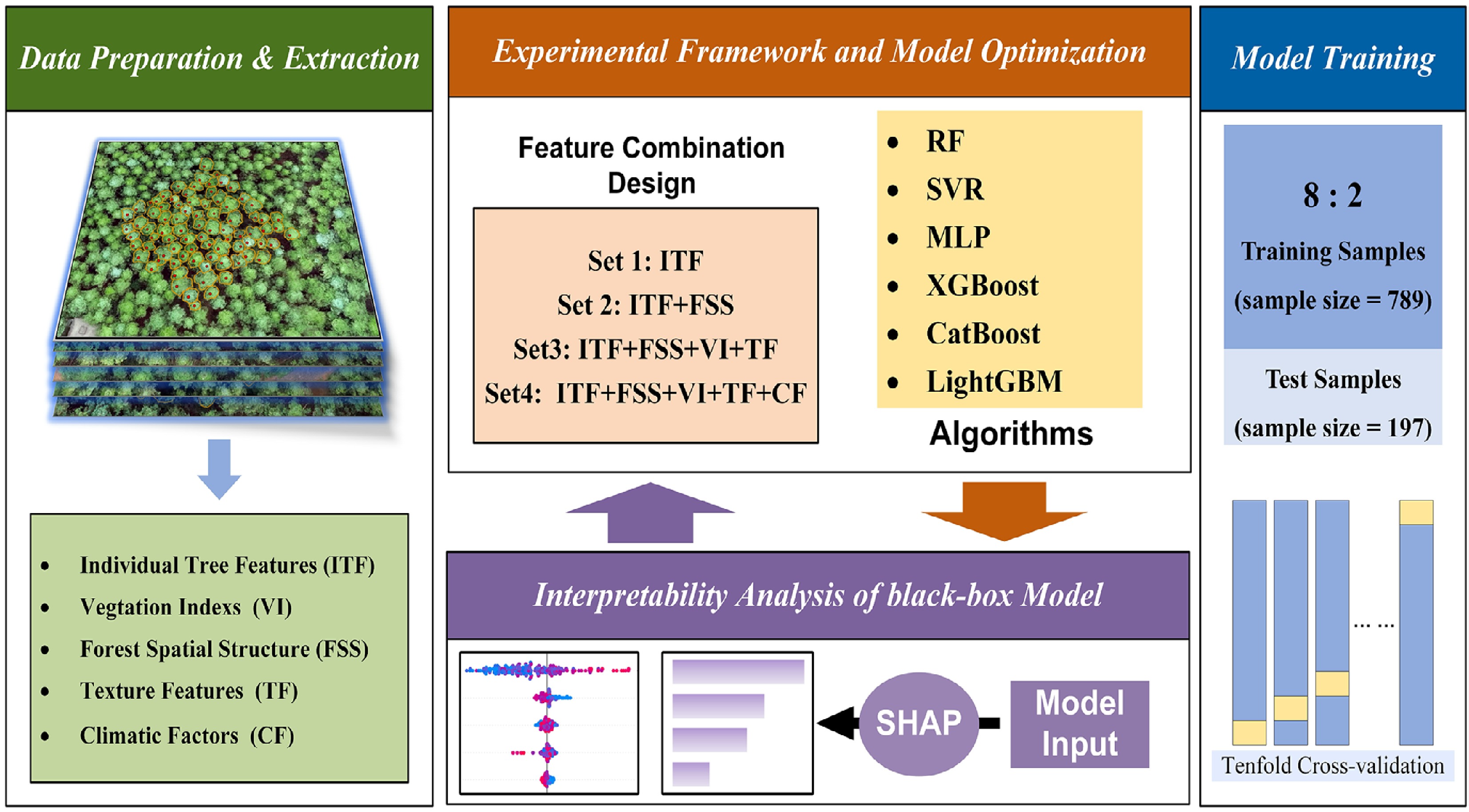
Figure 3.
Experimental framework and model optimization for DBH estimation.
-
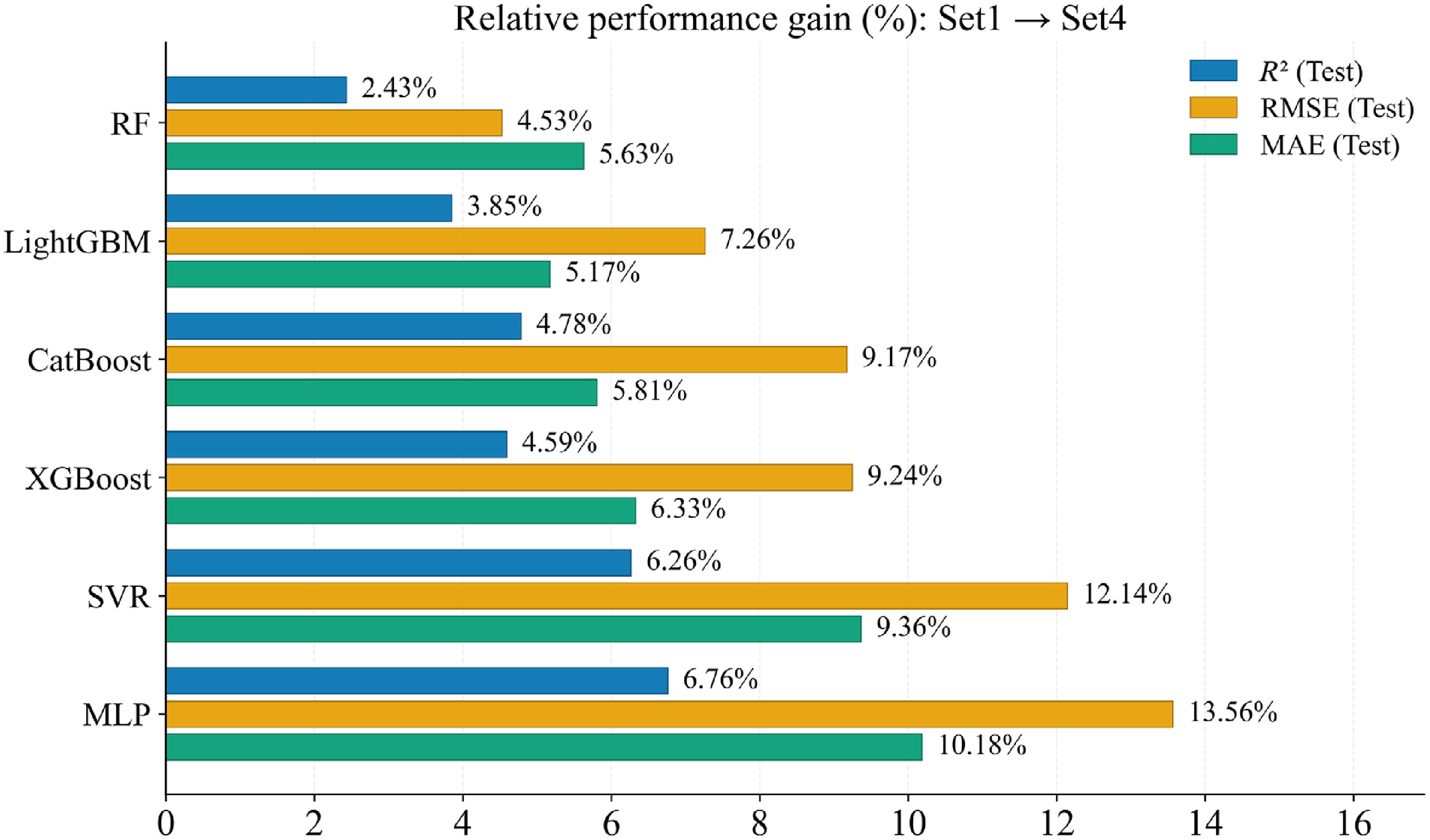
Figure 4.
Comparison of performance gains from feature fusion across models.
-
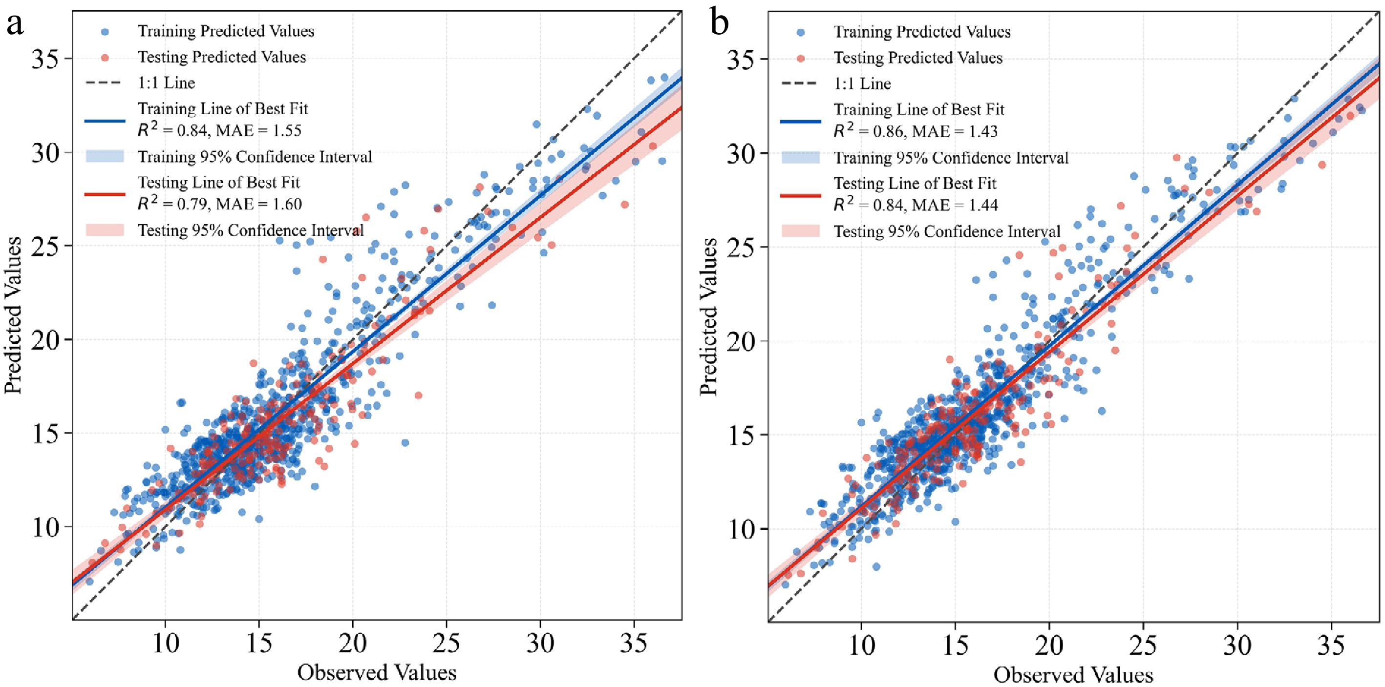
Figure 5.
Observed vs predicted DBH scatter plots for the MLP model under Set 1 and Set 4.
-
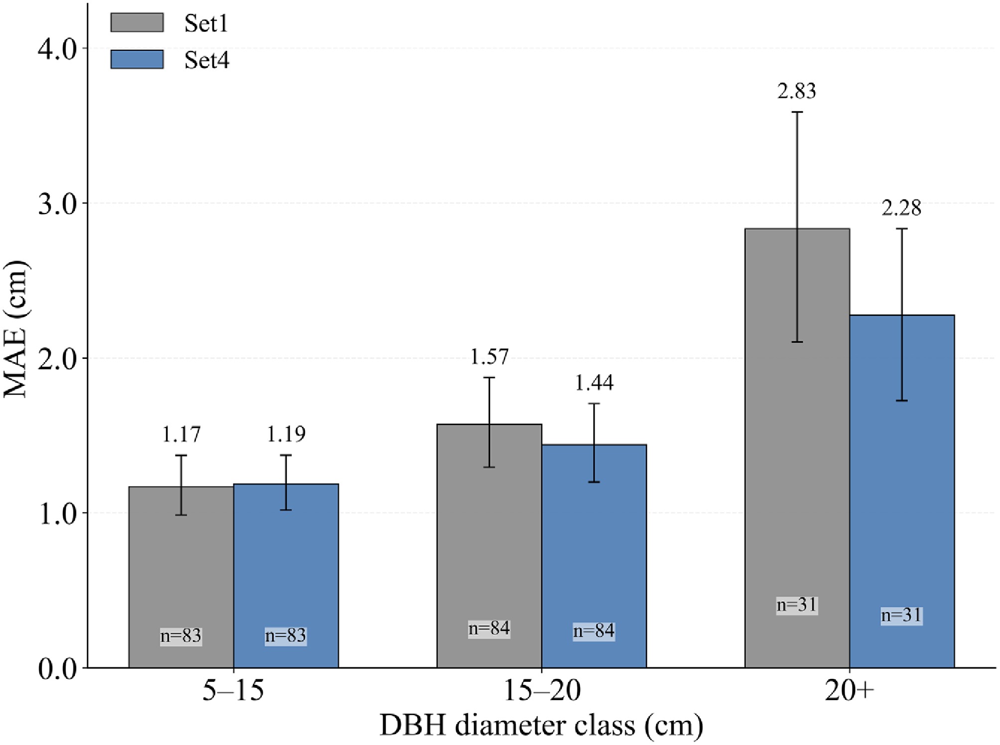
Figure 6.
MAE of the MLP model across DBH diameter classes for Set 1 and Set 4; n denotes sample size, and error bars represent 95% bootstrap confidence intervals.
-
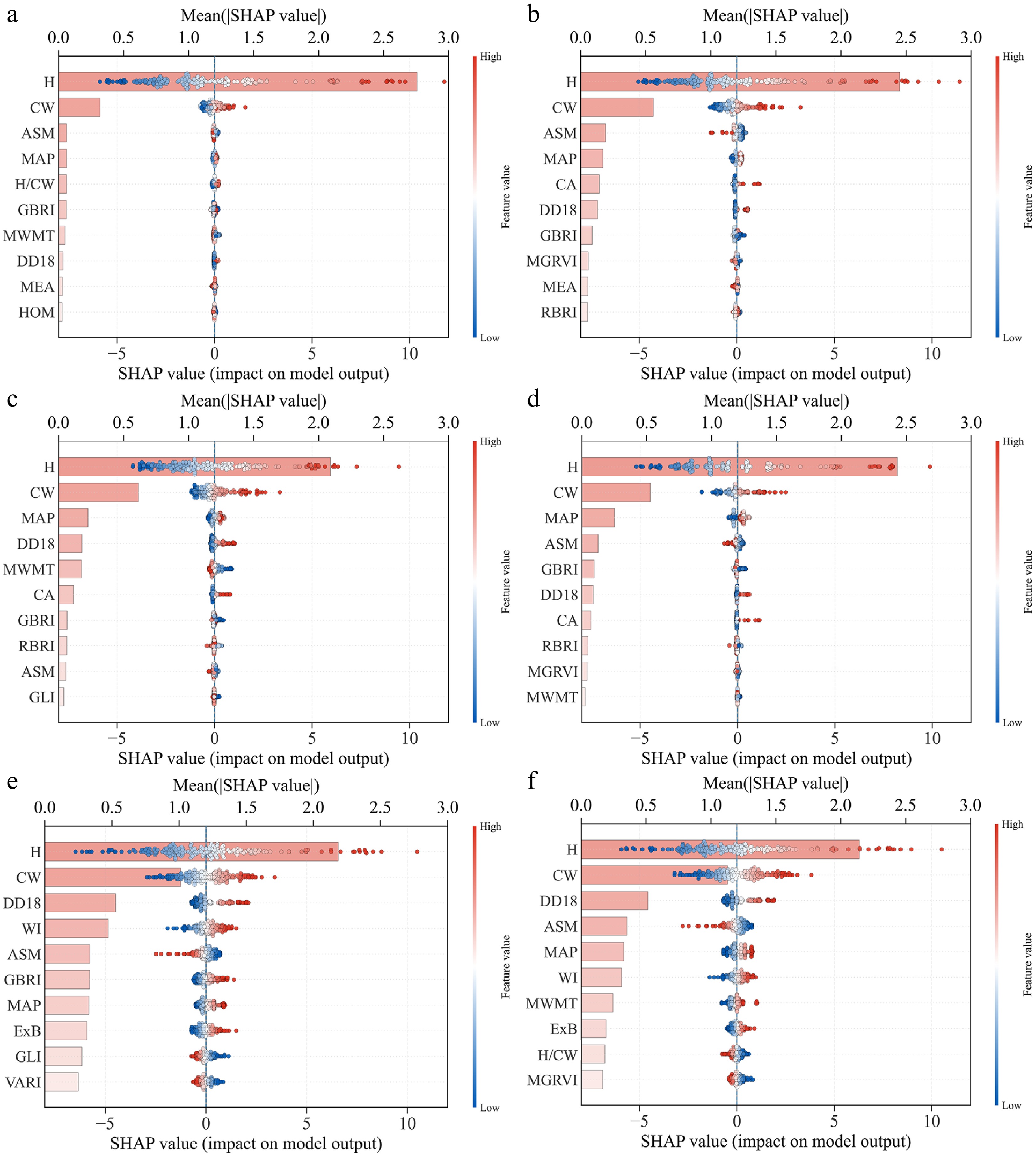
Figure 7.
SHAP summary plots for six machine-learning models under Set 4, showing the top 10 predictors ranked by mean |SHAP| (color indicates feature value from low to high).
-
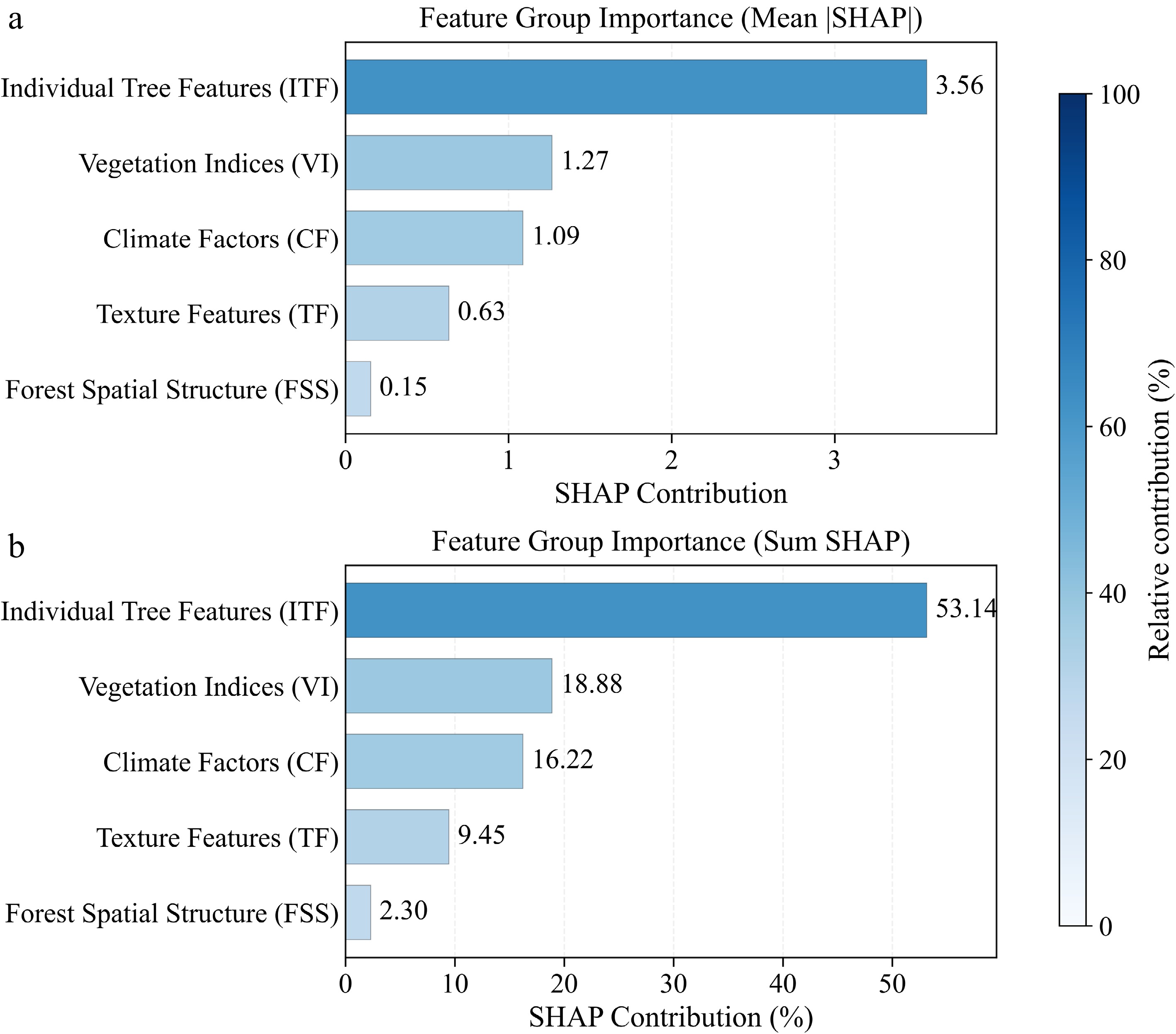
Figure 8.
Feature-group SHAP contributions for the MLP model under Set 4: (a) mean |SHAP|, and (b) summed SHAP contribution (%).
-
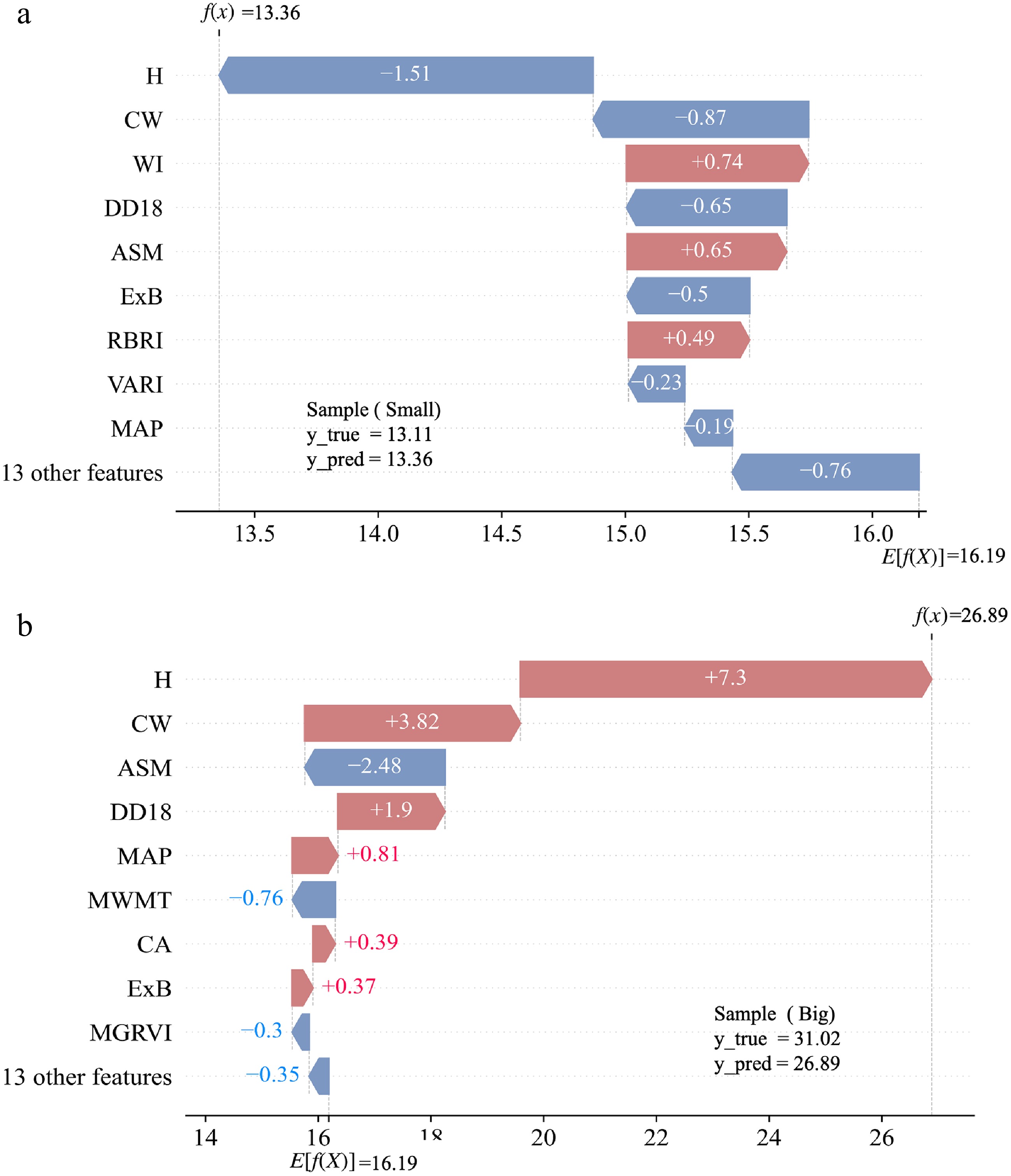
Figure 9.
SHAP waterfall plots for two representative samples: (a) small-DBH case, and (b) large-DBH case.
-
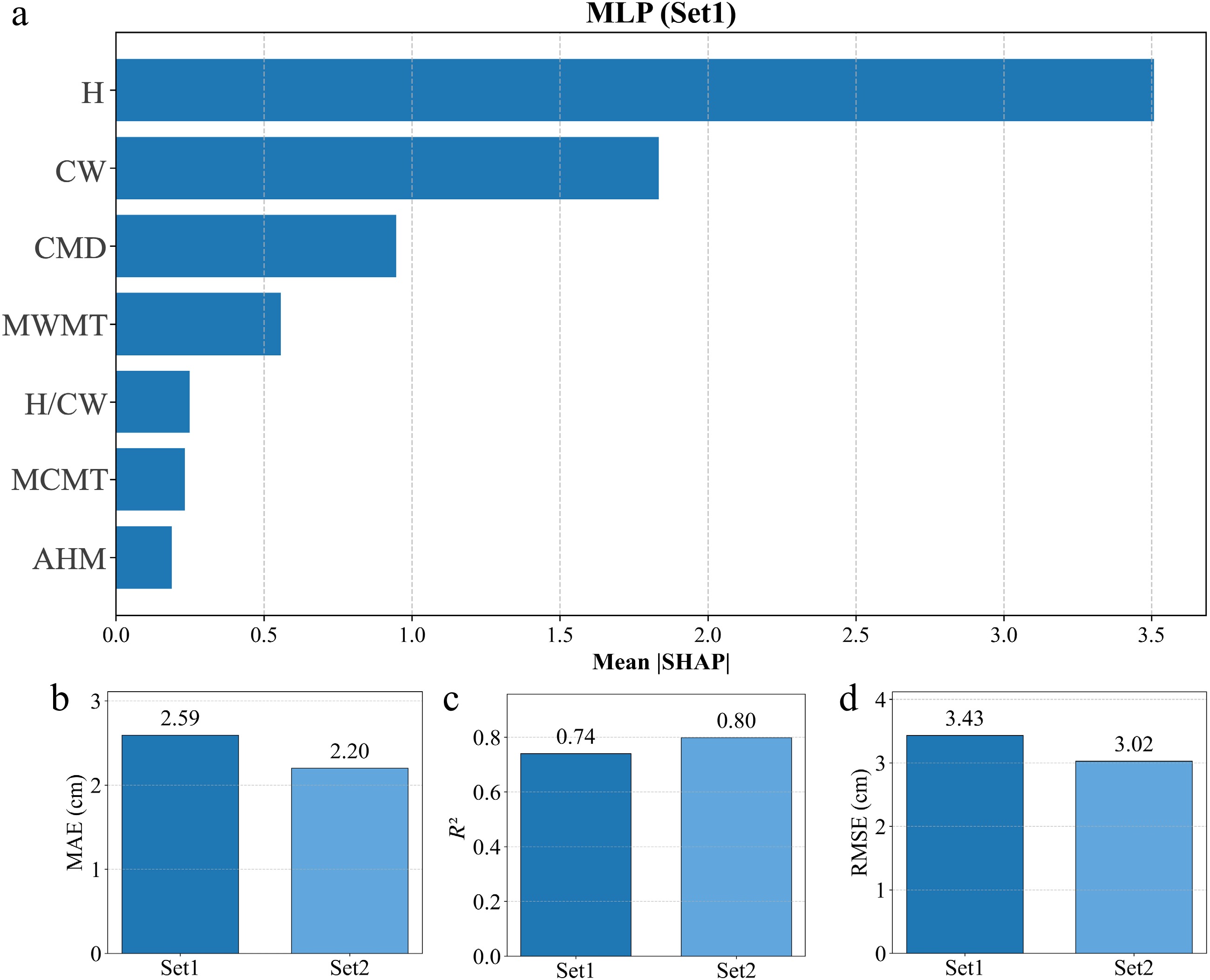
Figure 10.
Within-distribution performance comparison with climatic factors and feature-importance rankings.
-
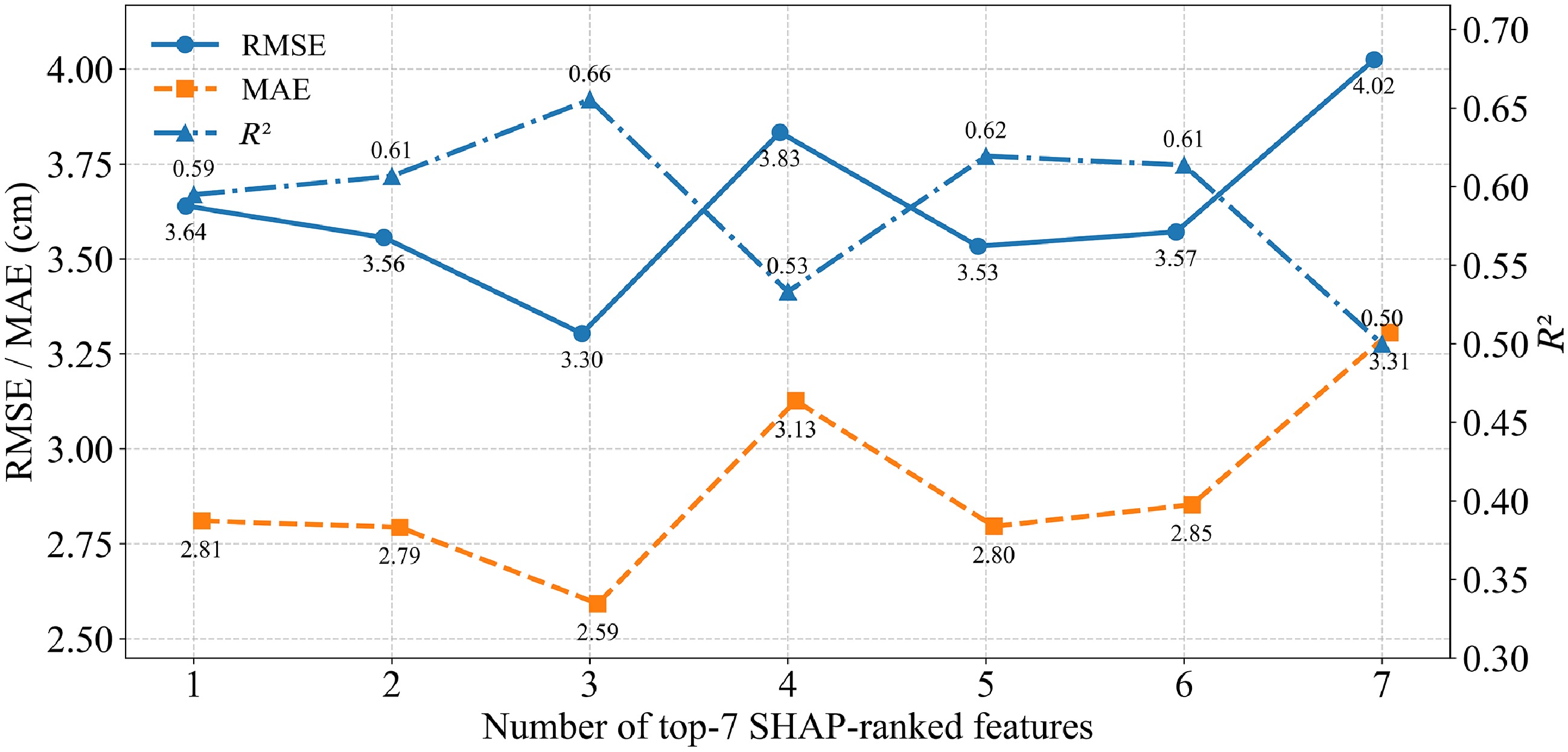
Figure 11.
Under LOSO extrapolation, MLP performance as top-ranked features are progressively incorporated.
-
Dataset Number of images Numbers of crowns Train 348 43,848 Validation 116 20,548 Test 116 19,738 Table 1.
Dataset split for crown instance segmentation.
-
VI Name Algorithm formula VARI Visible atmospherically resistant index $ (g-r)/(g+r-b) $ ExR Excess red vegetation index $ 1.4r-g $ ExB Excess blue vegetation index $ 1.4b-g $ ExG Excess Green Vegetation Index $ 2g-r-b $ GBRI Green–blue ratio index $ g/b $ RBRI Red–blue ratio index $ r/b $ WI Woebbecke index $ (g-b)/(r-g) $ GLI Green leaf index $ (2g-b-r)/(2g+b+r) $ NDI Normalized difference index $ (r-g)/(r+g+0.01) $ MGRVI Modified green red vegetation index $ ({g}^{2}-{r}^{2})/({g}^{2}+{r}^{2}) $ Table 2.
Summary of vegetation indices derived from orthorectified images of a drone used to estimate the DBH of Chinese fir.
-
TF Texture features Algorithm formula MEA Mean $ mea=\displaystyle\sum \limits_{i,j}^{N-1}{iP}_{i,j} $ VAR Variance $ var=\displaystyle\sum \limits_{i,j=0}^{N-1}{iP}_{i,j}{(i-mea)}^{2} $ HOM Homogeneity $ hom=\displaystyle\sum \limits_{i,j=0}^{N-1}i\dfrac{{P}_{i,j}}{1+{i-j}^{2}} $ CON Contrast $ con=\displaystyle\sum \limits_{i,j=0}^{N-1}i{P}_{i,j}{(i-j)}^{2} $ DIS Dissimilarity $ dis=\displaystyle\sum \limits_{i,j=0}^{N-1}i{P}_{i,j}\left| i-j\right| $ ENT Entropy $ ent=\displaystyle\sum \limits_{i,j=0}^{N-1}i{P}_{i,j}\left(-\ln {P}_{i,j}\right) $ ASM Angular second moment $ asm=\displaystyle\sum \limits_{i,j=0}^{N-1}i{{{P}^{2}}}_{i,j} $ COR Correlation $ cor=\displaystyle\sum \limits_{i,j=0}^{N-1}i{P}_{i,j}\left[\dfrac{(i-mea)(j-mea)}{\sqrt{{var}_{i}*{var}_{j}}}\right] $ Table 3.
Textural index used in this study.
-
Model Hyper-parameter values RF max_samples: 0.2, 0.5, 0.8;
max_depth:1, 5, 10, 15;
min_samples_split: 2, 5, 7, 10XGBoost max_depth: 3, 5, 10, 15;
reg_lambda: 0.1, 0.5, 1, 2;
min_child_weight: 1, 5, 10, 15;
learning_rate: 0.001, 0.01, 0.1, 0.05CatBoost depth: 3, 5, 7, 10;
subsample: 0.2, 0.5, 0.8;
min_data_in_leaf: 1, 3, 5, 10;
learning_rate: 0.001, 0.01, 0.1, 0.5LightGBM subsample: 0.2, 0.5, 0.8;
max_depth: −1, 5, 10, 15;
num_leaves: 5, 10, 15, 20;
min_child_sample: 5, 10, 15, 20;
learning_rate: 0.001, 0.01, 0.1, 0.05SVR gamma: scale, auto;
kernel: rbf, sigmoid;
epsilon: 0.1, 0.3, 0.5, 0.7;
C: 0.1, 1, 10, 50, 90, 100, 110MLP solver: adam, sgd;
alpha: 0.01, 0.1, 1, 2, 5, 10;
learning_rate_init: 0.1, 0.01, 0.001, 0.05;
hidden_layer_sizes: (64, ), (64, 32), (128, ), (128,64), (128, 64, 32),
(128, 65, 32, 16)Table 4.
The hyperparameters for each model have been predetermined through a grid search.
-
Model Set 1 Set 2 Set 3 Set 4 R2 RMSE (cm) MAE (cm) R2 RMSE (cm) MAE (cm) R2 RMSE (cm) MAE (cm) R2 RMSE (cm) MAE (cm) RF 0.78 2.15 1.63 0.78 2.16 1.63 0.79 2.11 1.58 0.81 2.06 1.54 XGBoost 0.79 2.11 1.59 0.80 2.10 1.59 0.82 1.99 1.52 0.83 1.91 1.49 CatBoost 0.79 2.15 1.61 0.79 2.13 1.60 0.81 2.05 1.54 0.82 1.95 1.51 LightGBM 0.78 2.16 1.61 0.78 2.11 1.60 0.80 2.10 1.59 0.82 1.98 1.52 SVR 0.78 2.15 1.63 0.79 2.11 1.59 0.81 2.0 1.54 0.83 1.89 1.48 MLP 0.79 2.13 1.60 0.80 2.08 1.59 0.82 1.98 1.51 0.84 1.84 1.44 Ave 0.79 2.14 1.61 0.79 2.13 1.60 0.81 2.04 1.55 0.82 1.94 1.50 Table 5.
Evaluation metrics results for each model for four feature combination sets.
Figures
(11)
Tables
(5)