-
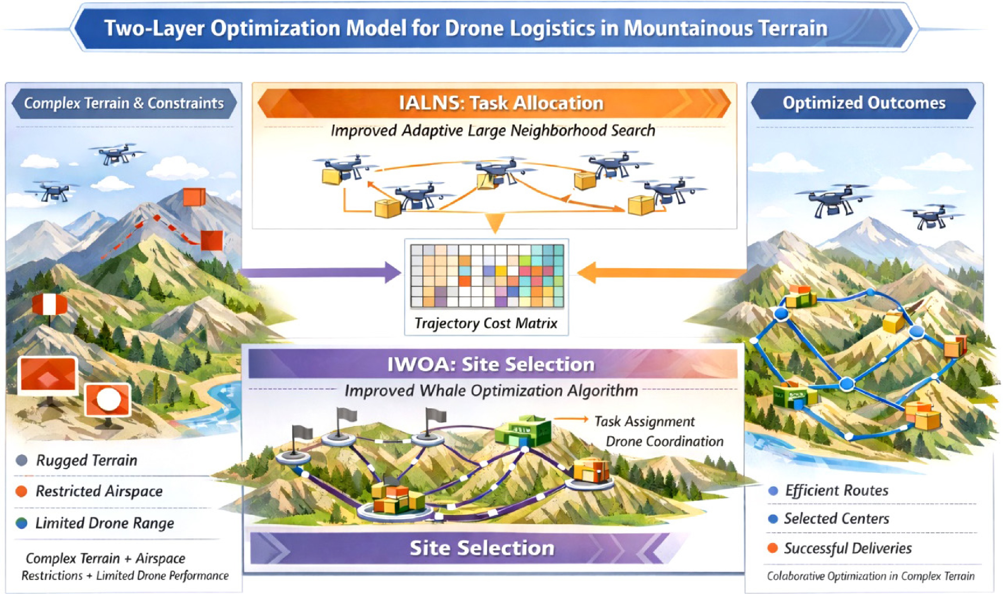
Figure 1.
Research model diagram.
-
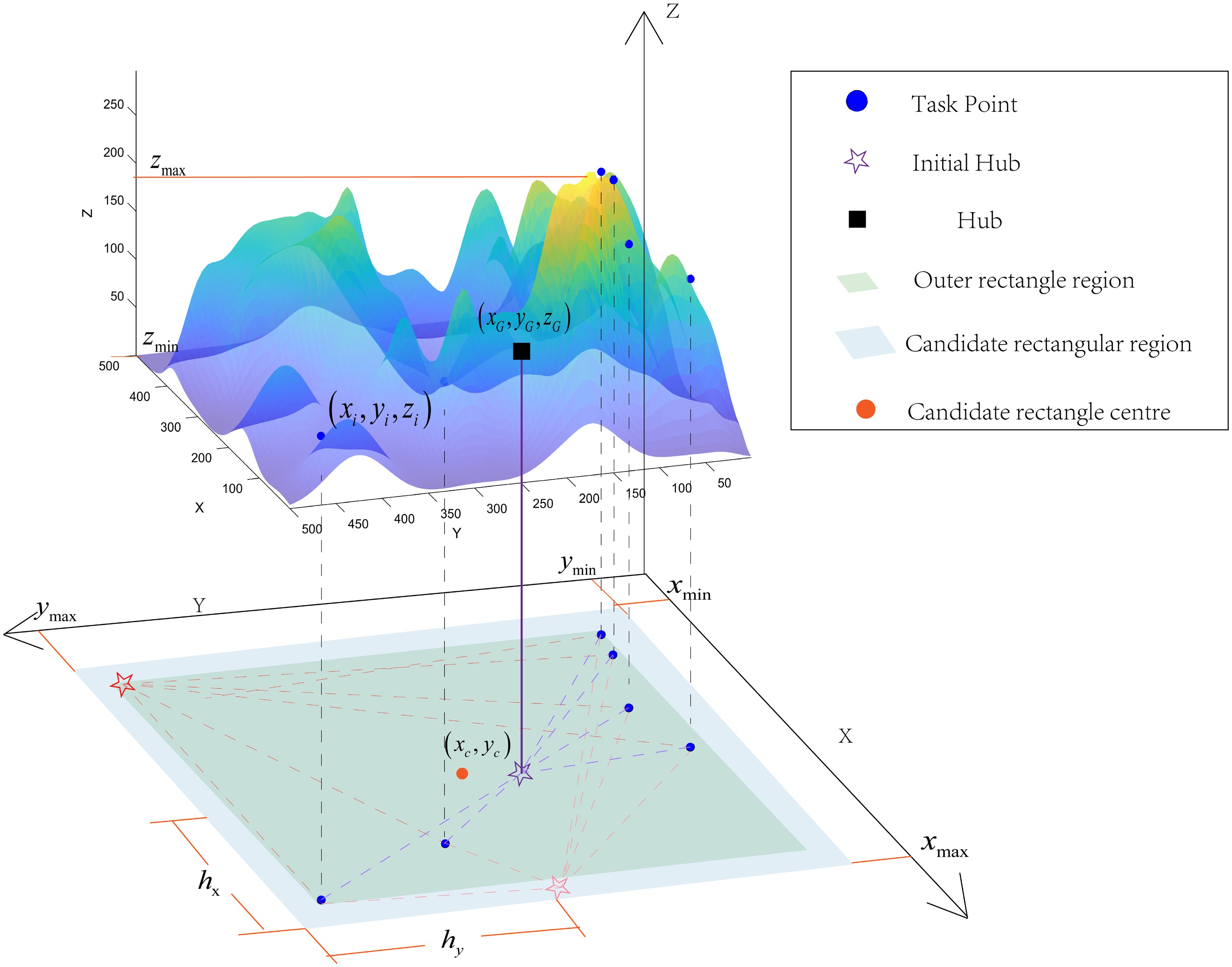
Figure 2.
Hub selection schematic.
-
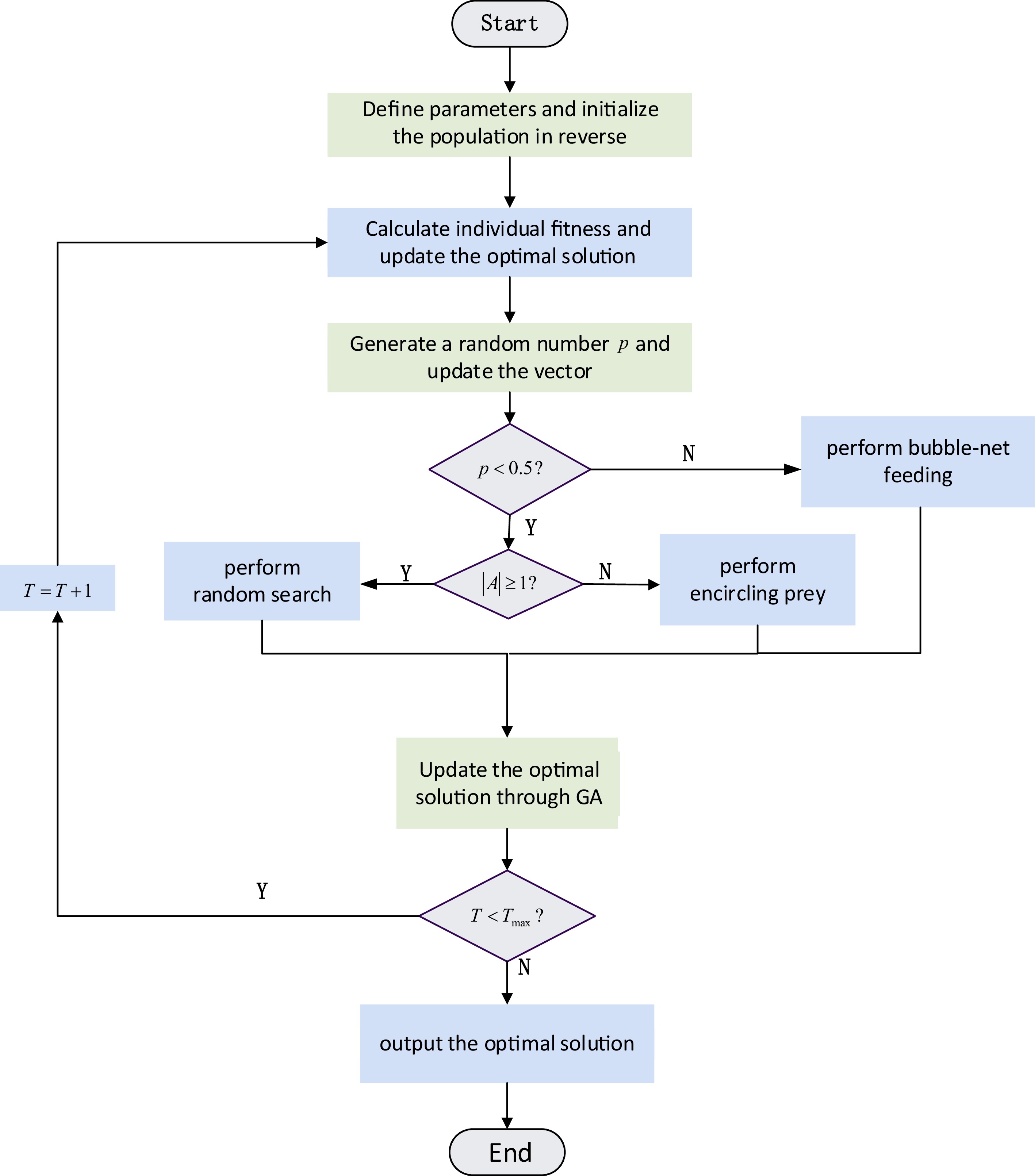
Figure 3.
Flow chart of IWOA. The modules marked in green correspond to the improvement mechanism, while the remaining modules follow the standard WOA process.
-
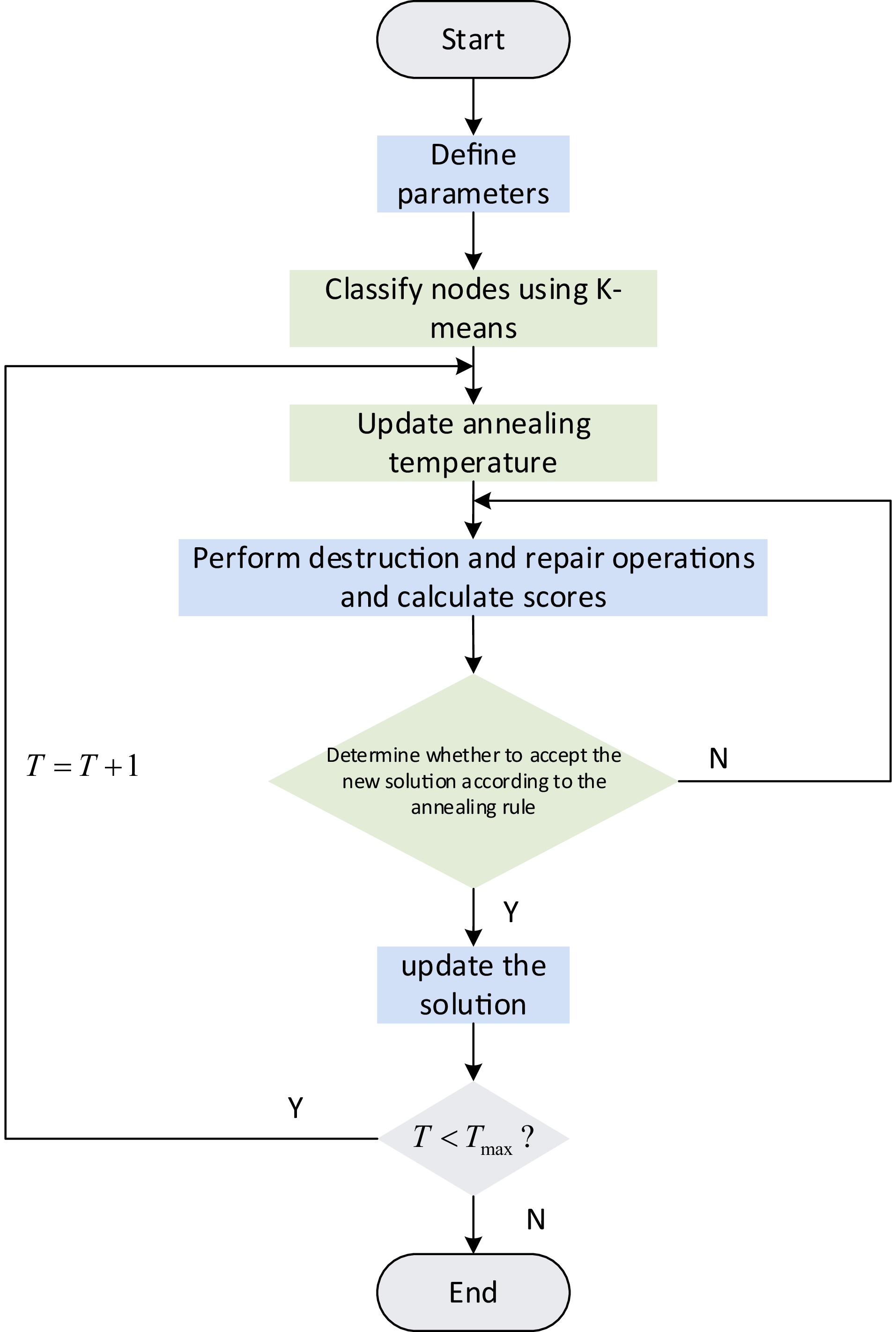
Figure 4.
Flowchart of IALNS. The modules marked in green correspond to the improvement mechanism, while the remaining modules follow the standard ALNS process.
-
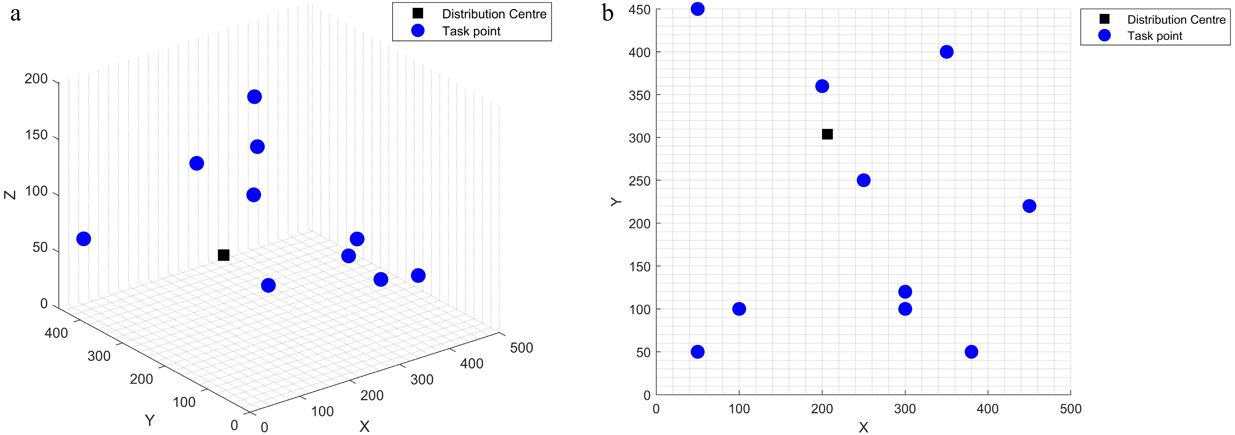
Figure 5.
Hub location schematic. (a) Side view of spatial distribution. (b) Top view of spatial distribution.
-
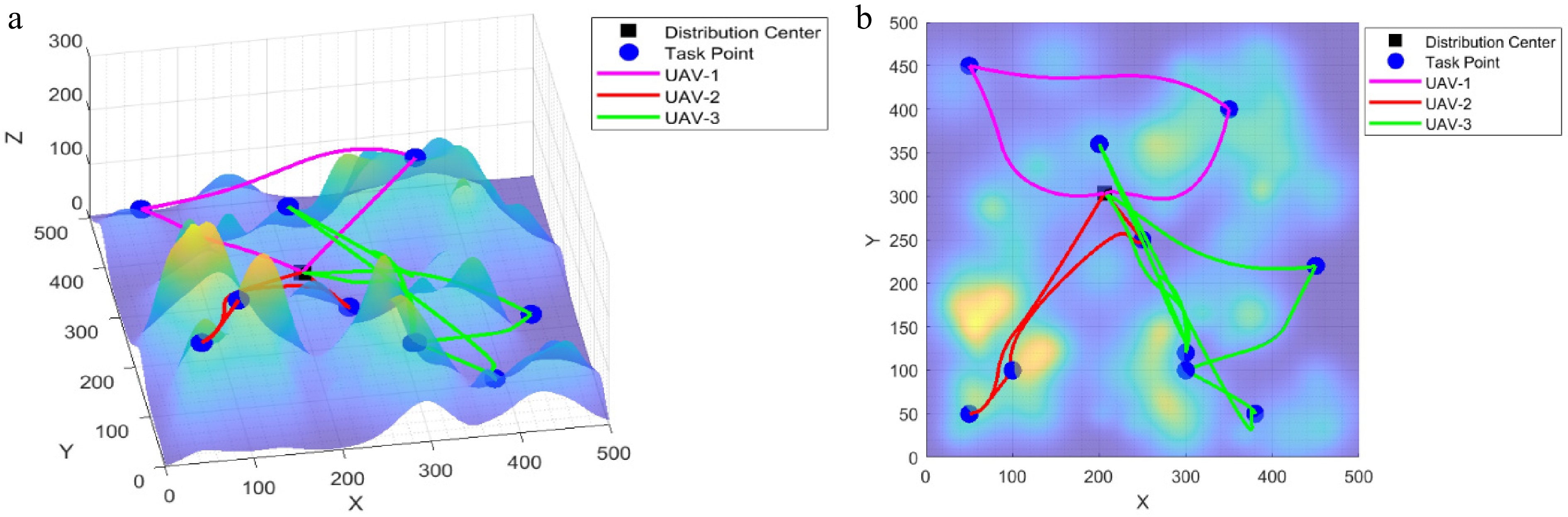
Figure 6.
Planned trajectory diagram of WOA–ALNS; (a) side view, and (b) top view.
-
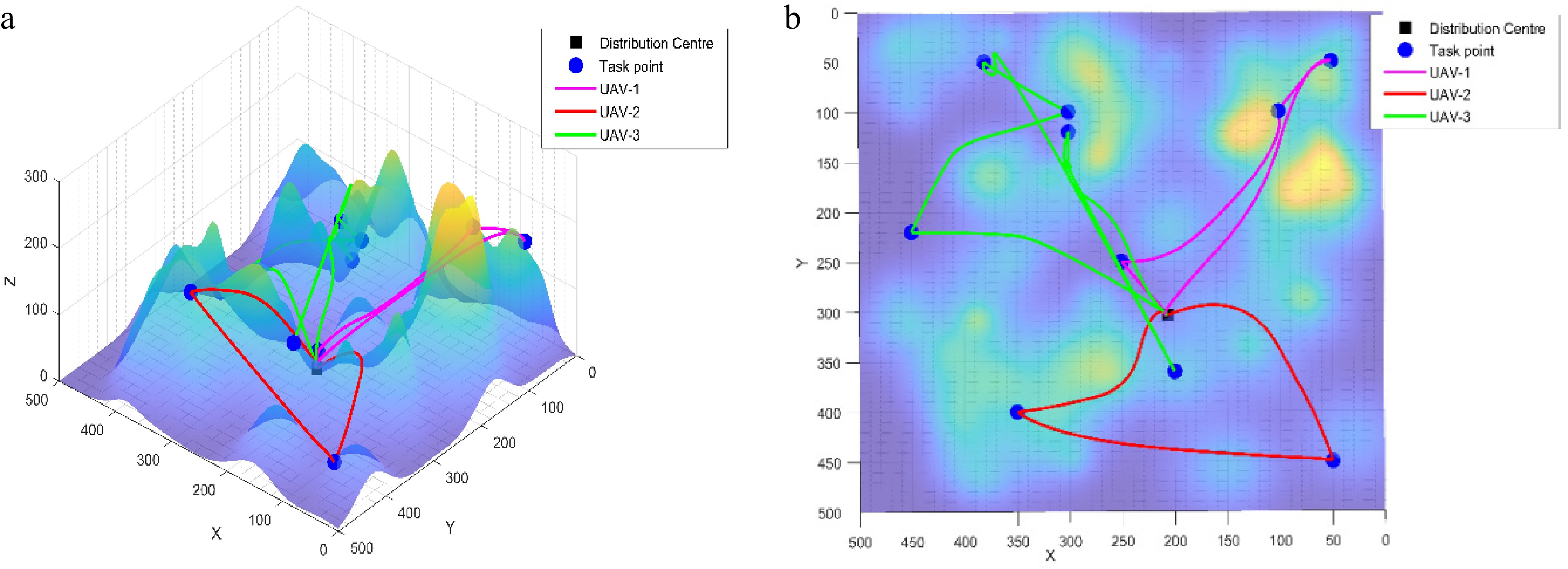
Figure 7.
Planned trajectory diagram of IWOA–IALNS; (a) side view, and (b) top view.
-
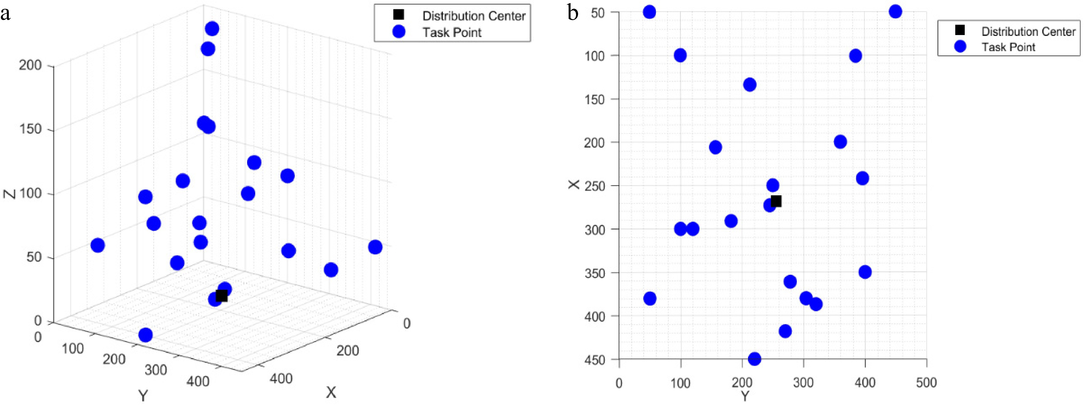
Figure 8.
Hub location schematic; (a) side view of spatial distribution, and (b) top view of spatial distribution.
-
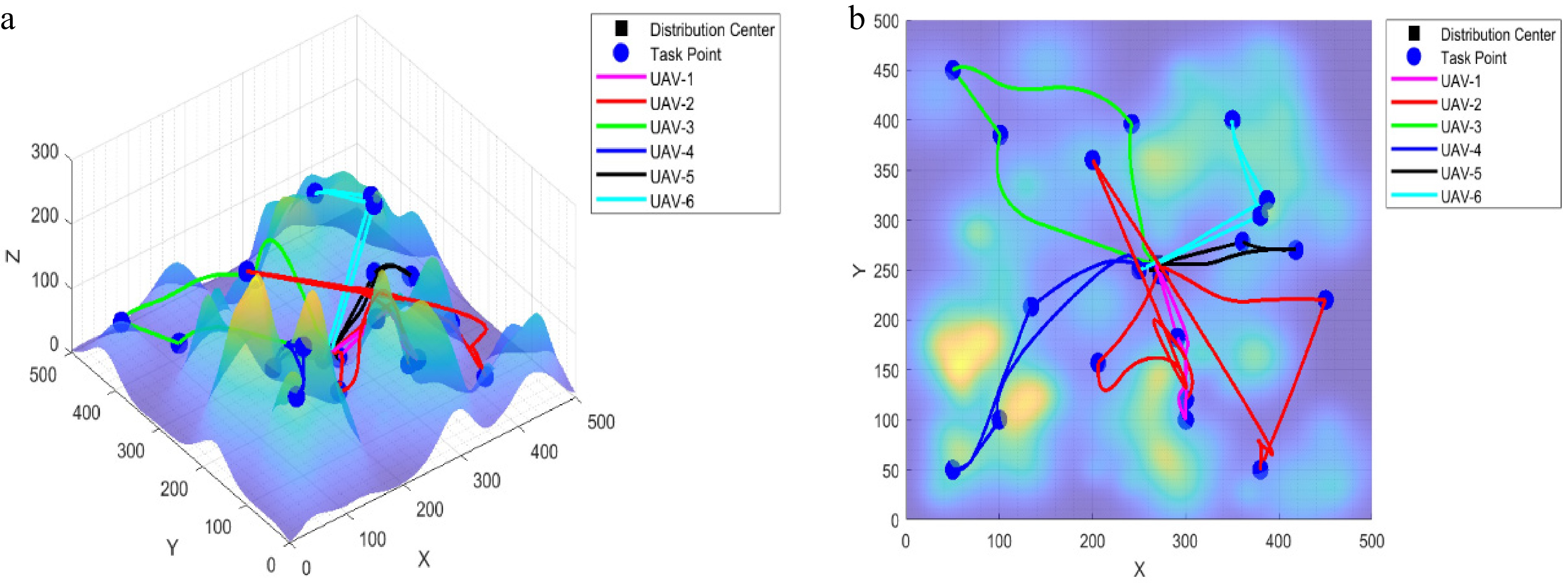
Figure 9.
Planned trajectory diagram of WOA–ALNS; (a) side view, and (b) top view.
-
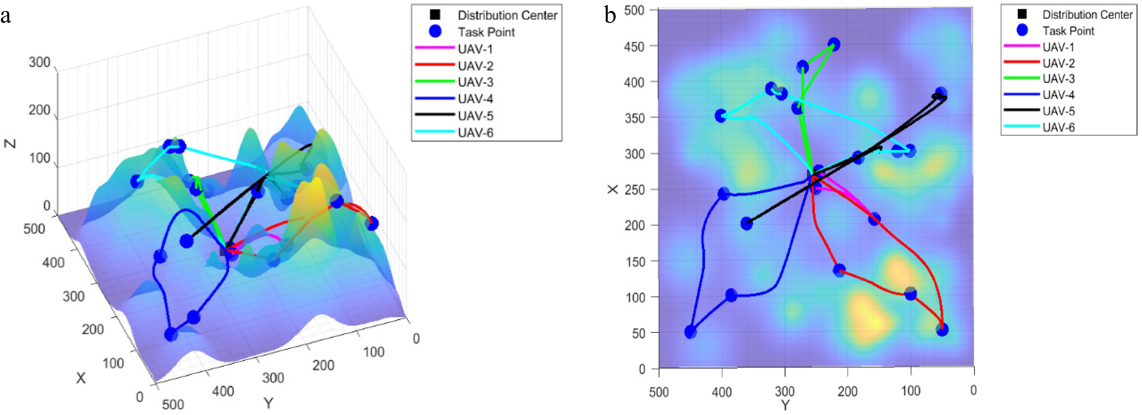
Figure 10.
Planned trajectory diagram of IWOA–IALNS; (a) side view, and (b) top view.
-
Vehicle Research scenario Dual-Layer algorithm Primary constraints Ref. Vehicle trajectory Vehicle merging Upper layer: DRL generates initial trajectory.
Lower layer: MPC refines trajectory.Risk; collision; dynamics Wu et al.[15] Electric bus vehicles Urban mobility Upper layer: ALNS planning and operations benefits.
Lower layer: VNS computing charging costs.Energy; charging; profitability Jiang et al.[16] Drone Urban airspace Upper layer: 3D flight path.
Lower layer: time dimension conflict resolution.Urban risk; conflict; time dimension Zheng et al.[17] Drone Urban airspace Upper layer: generate candidate solutions.
Lower layer: resolve 4-time dimension conflicts.Risk; conflict; timeliness Chen et al.[18] Logistics drones Urban airspace Upper layer: takeoff and landing point layout.
Lower layer: flight route planning.Coverage requirements; facility construction Zhang et al.[19] Table 1.
Comparative table of related studies.
-
Type Variable symbol Variable meaning Assembly $ I $ Task point collection, $ I=\left\{1,2,3,\cdot \cdot \cdot ,n\right\} $ $ L $ Waypoint set, $ L=\left\{1,2,3,\cdot \cdot \cdot ,m\right\} $ $ V $ Task points and hub points collection, where 0 denotes the distribution center. $ V=\left\{0,1,2,\cdot \cdot \cdot ,a\right\} $ $ K $ Drones assemble. $ K=\left\{1,2,3,\cdots ,b\right\} $ Parameters $ \left({x}_{G},{y}_{G},{z}_{G}\right) $ Coordinates of the distribution center requiring optimization $ i=\left({x}_{i},{y}_{i},{z}_{i}\right) $ Task point coordinates $ {d}_{i} $ The straight-line distance between task point $ i $ $ {L}_{i} $ The Euclidean distance between waypoint $ l $ $ l+1 $ $ {q}_{i} $ Task volume at point $ i $ $ {p}_{c} $ The maximum operational workload that a drone can handle (kg) $ {w}_{i} $ Time of arrival at Task Point $ i $ $ \begin{array}{cc}{w}_{i,1}, & {w}_{i,2}\end{array} $ The left and right time windows at Task Point $ i $ $ \begin{array}{cc}{x}_{\max }, & {x}_{\min }\end{array} $ Upper and lower bounds of the candidate rectangle's x-boundary (km) $ \begin{array}{cc}{y}_{\max }, & {y}_{\min }\end{array} $ Upper and lower bounds of the candidate rectangle's y-boundary (km) $ \left({x}_{c},{y}_{c}\right) $ Candidate rectangle center $ \begin{array}{cc}{h}_{\mathrm{x}}, & {h}_{y}\end{array} $ The half-width and half-length of a rectangular boundary $ \begin{array}{cc}{z}_{\max }, & {z}_{\min }\end{array} $ Upper and lower limits of terrain surface elevation (km) $ \begin{array}{cc}{B}_{\max }, & {B}_{\min }\end{array} $ Upper and lower limits for distribution center construction costs (CNY) $ \rho $ Offset between the distribution center and the candidate rectangle center $ \delta $ Cost item weighting in the site selection model $ \alpha $ Cost weighting for site selection and flight path planning layer $ \omega $ Task allocation layer cost item weighting Decision Variable $ x_{ij}^{k}\in \left\{0,1\right\} $ When drone $ k $ $ i $ $ j $ $ x_{ij}^{k}=1 $ $ x_{ij}^{k}=0 $ $ {y}_{g}\in \left\{0,1\right\} $ When selecting candidate point $ {g}_{} $ $ {y}_{g}=1 $ $ {y}_{m}=0 $ Table 2.
Variable symbols and their meanings.
-
Task point number Coordinates Time window Service hours Workload 1 (50, 50) (600, 630) 20 40 2 (380, 50) (570, 600) 20 10 3 (50, 450) (60, 150) 20 40 4 (450, 220) (540, 570) 20 10 5 (250, 250) (20, 60) 20 20 6 (100, 100) (480, 520) 20 10 7 (200.360) (160, 200) 20 40 8 (350.400) (220, 270) 20 30 9 (300, 100) (460, 500) 20 10 10 (300, 120) (300, 330) 20 5 11 (273, 245) (160, 250) 20 40 12 (101, 385) (50, 90) 20 20 13 (242, 396) (94, 144) 20 30 14 (380, 304) (567, 597) 20 5 15 (387, 320) (194, 254) 20 30 16 (418, 270) (144, 204) 20 40 17 (291, 182) (588, 630) 20 30 18 (134, 213) (219, 269) 20 20 19 (361, 278) (589, 630) 20 30 20 (206, 157) (258, 318) 20 20 Table 3.
Starting and ending point coordinate information.
-
Performance indicators Parameters Maximum load 110 Safety height 5 Cruising speed 10 Table 4.
Drone configuration information.
-
Algorithm model Drone serial number Route task point number Workload Flight distance WOA–ALNS 1 Hub-3-8-Hub 70 762.9931 2 Hub-5-6-1-Hub 70 747.2684 3 Hub-10-7-2-9-4-Hub 75 1,645.1407 IWOA–IALNS 1 Hub-5-6-1-Hub 70 747.1739 2 Hub-3-8-Hub 70 732.6863 3 Hub-10-7-2-9-4-Hub 75 1,405.1481 Table 5.
Statistics on the performance of unmanned aerial vehicles.
-
Algorithm model Drone serial number Route task point number Workload Flight distance WOA–ALNS 1 Hub-11-9-17-Hub 80 376.6751 2 Hub-20-10-7-2-4-Hub 85 1,227.3709 3 Hub-12-3-13Hub 90 644.8365 4 Hub-18-1-6-Hub 70 723.4462 5 Hub-16-19-Hub 70 337.6873 6 Hub-5-15-8-14-Hub 85 622.632 IWOA–IALNS 1 Hub-5-20-11-Hub 80 252.0177 2 Hub-18-6-1-Hub 70 630.6304 3 Hub-16-4-19-Hub 80 491.9512 4 Hub-12-3-13-Hub 90 580.8365 5 Hub-10-7-2-17-Hub 85 859.4272 6 Hub-8-15-14-9-Hub 75 624.7721 Table 6.
Statistics on the performance of UAVs.
Figures
(10)
Tables
(6)