-
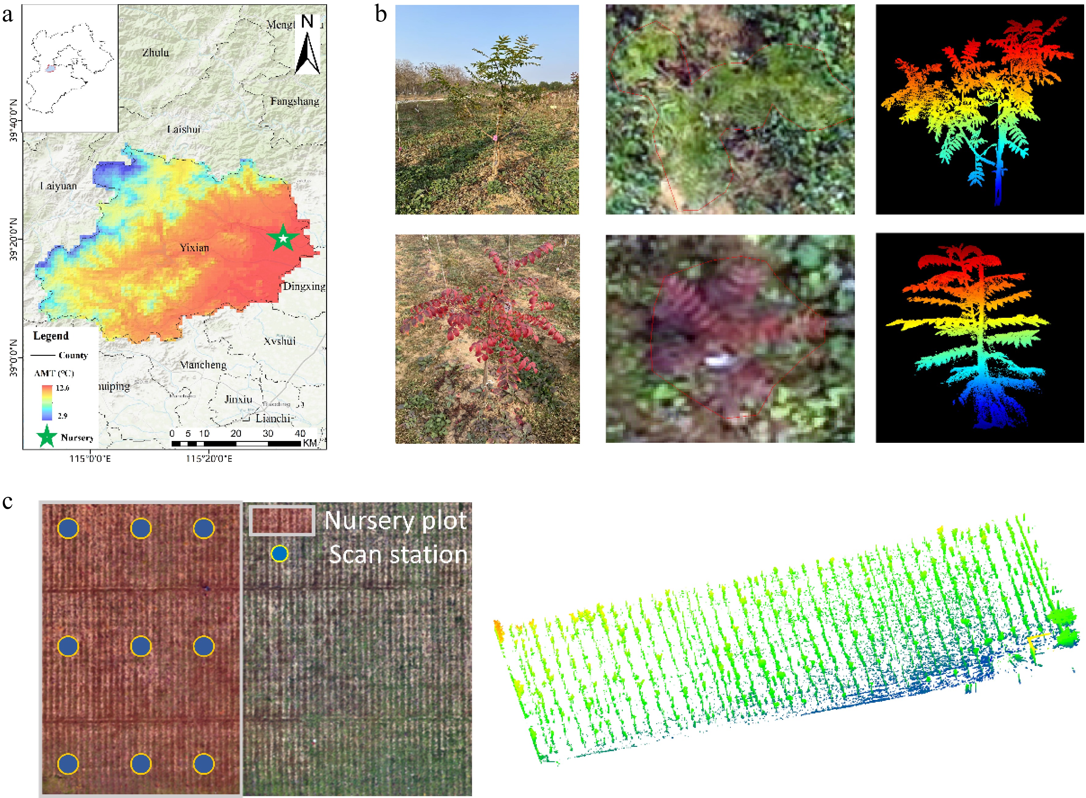
Figure 1.
(a) The experimental site of this study. (basemap source: Esri topographic map, generated using ArcGIS). (b) Example photos of cloned seedlings, UAV RGB orthophotos, and TLS point clouds. (c) The selected area in the Pistacia chinensis cloned seedling nursery, and the distribution of terrestrial laser scans (TLS), as well as single-station seedling TLS data.
-
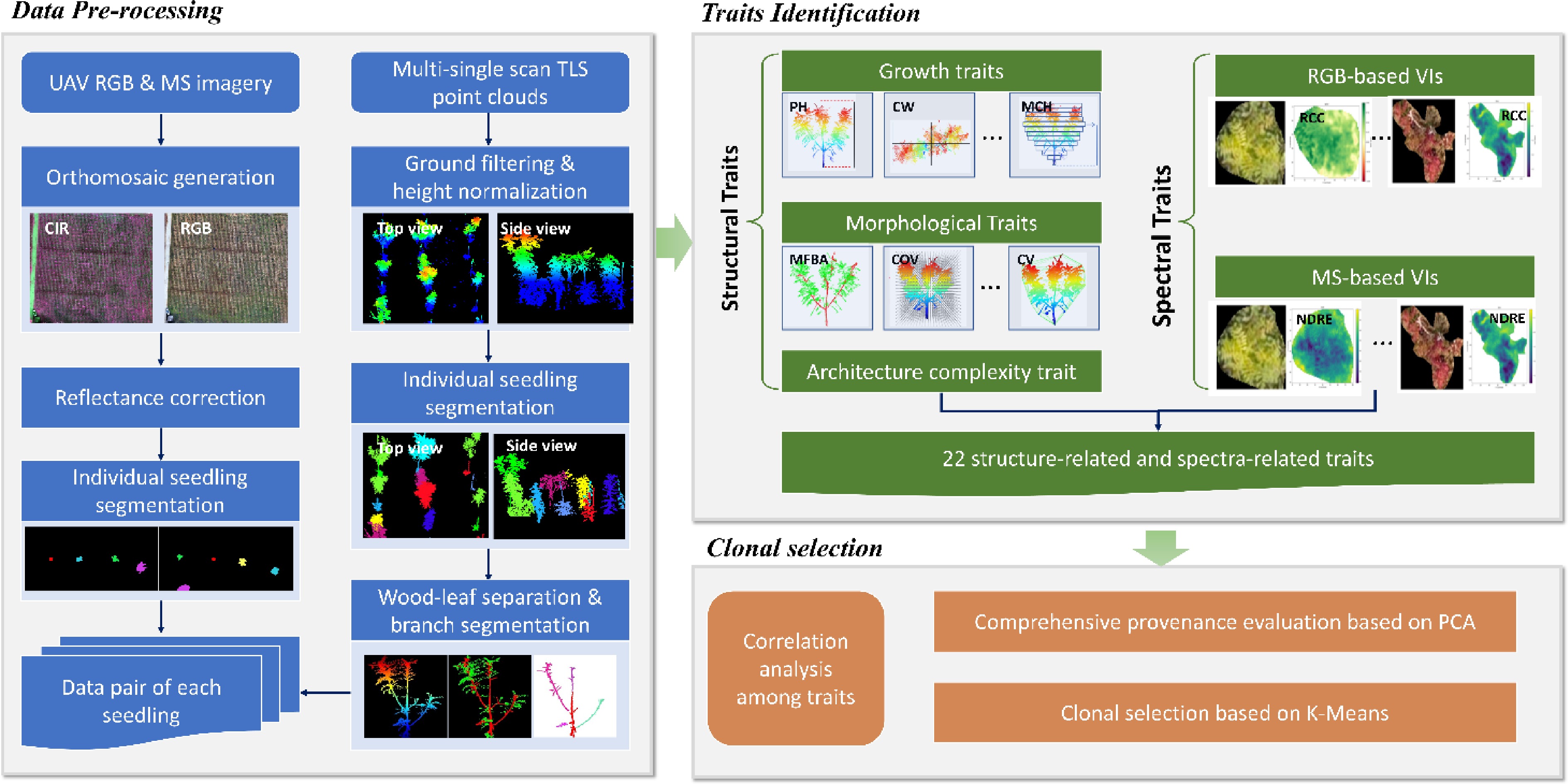
Figure 2.
Workflow diagram of the proposed multi-modal proximal sensing pipeline for seedling phenotyping. The workflow starts with TLS point cloud and UAV multispectral/RGB image acquisition, followed by stream-specific preprocessing, seedling-level processing, and finally outputs of structural- and spectral-trait tables for downstream analyses.
-
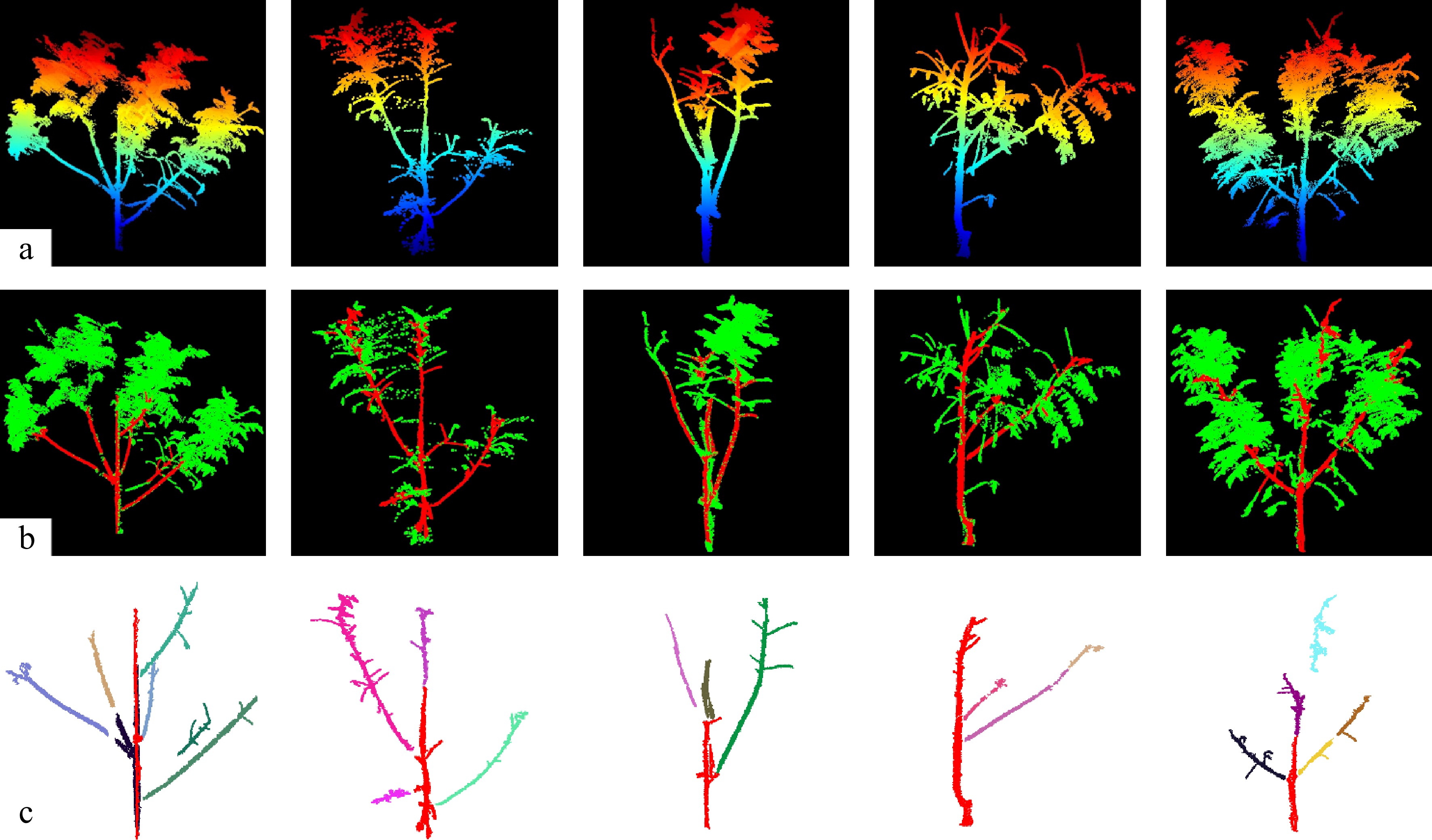
Figure 3.
(a) Visualization of representative Pistacia chinensis seedling point clouds, (b) separation of leaf and woody components, and (c) segmentation of the main stem and first-order branches, where different colors indicate different first-order branches.
-
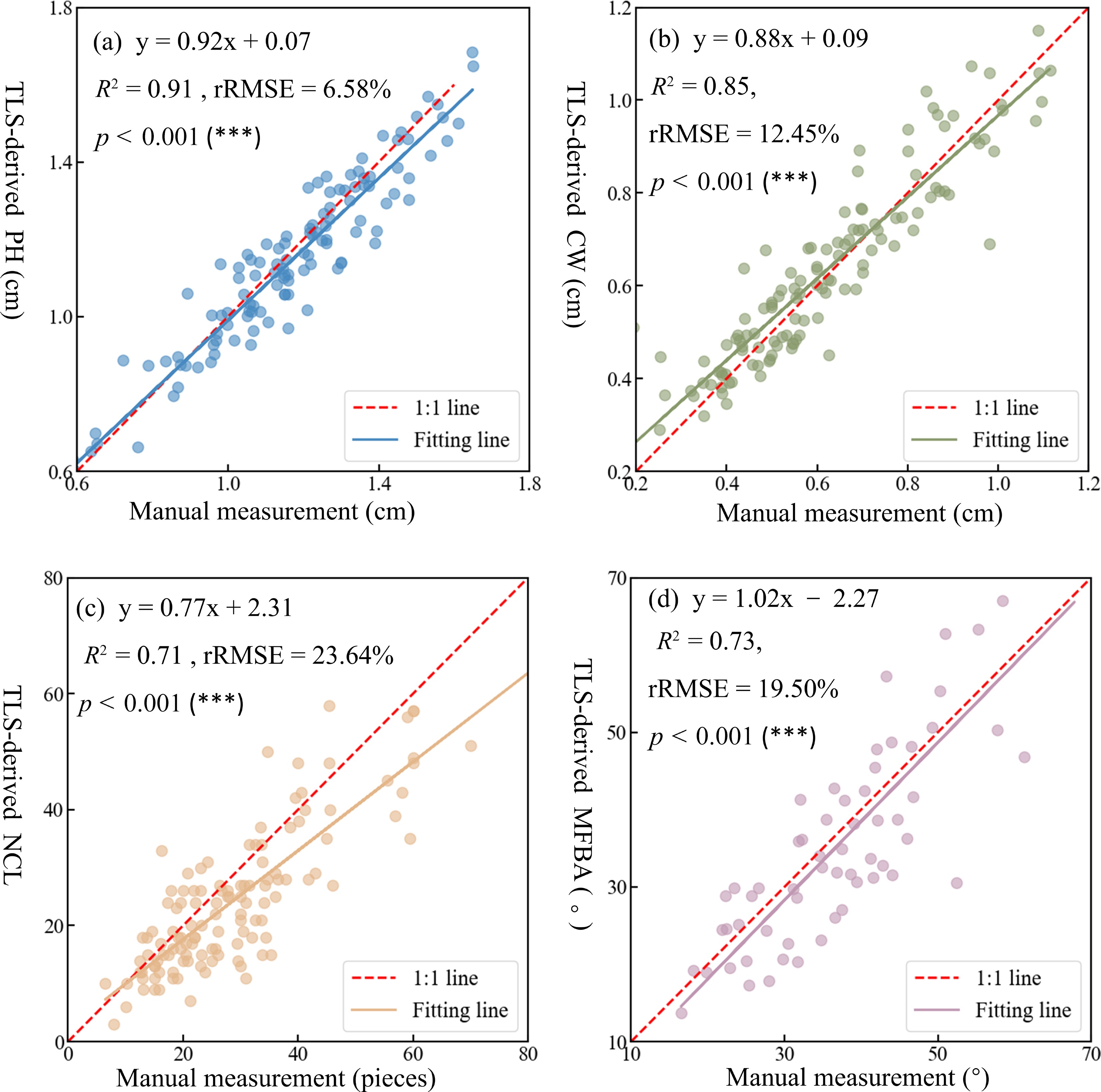
Figure 4.
Comparison between TLS-derived and manually-measured structural traits of Pistacia chinensis seedlings. (a) Plant height, (b) crown width, (c) number of compound leaves, and (d) mean of first-order branch angles.
-
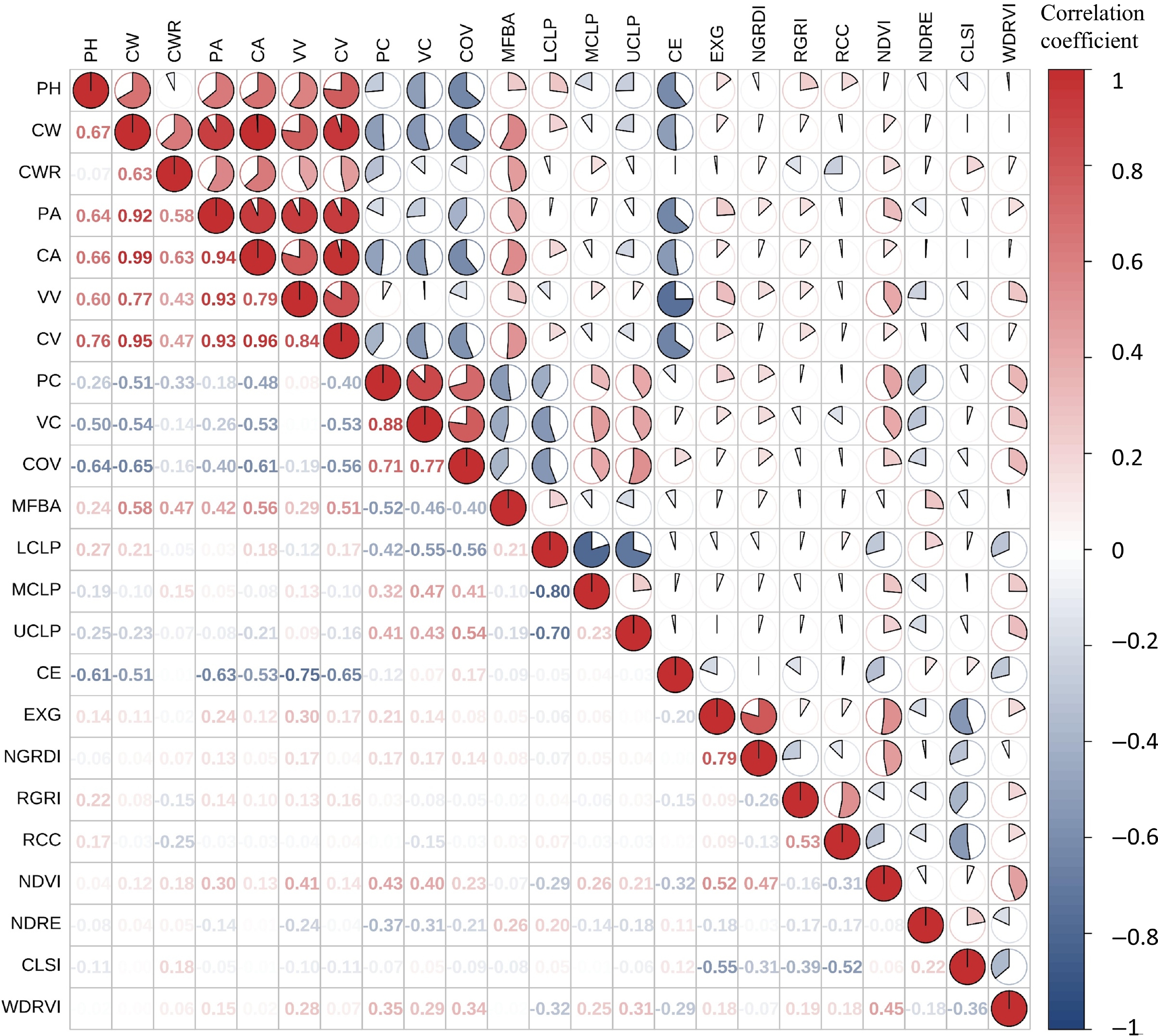
Figure 5.
Spearman's correlation analysis for structural and spectral traits of Pistacia chinensis seedlings.
-
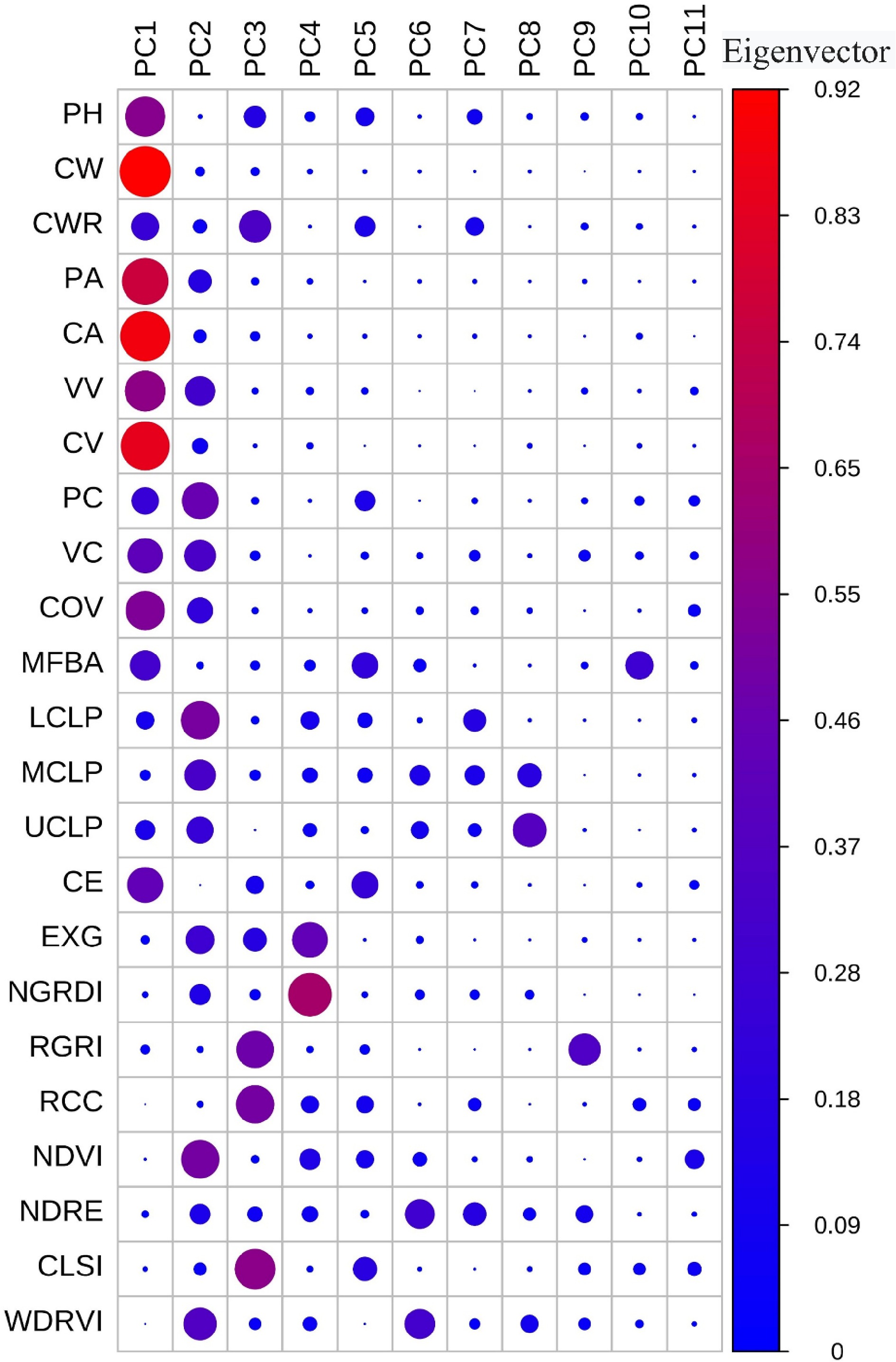
Figure 6.
Normalization of the structural and spectral traits of all seedlings using PCA.
-
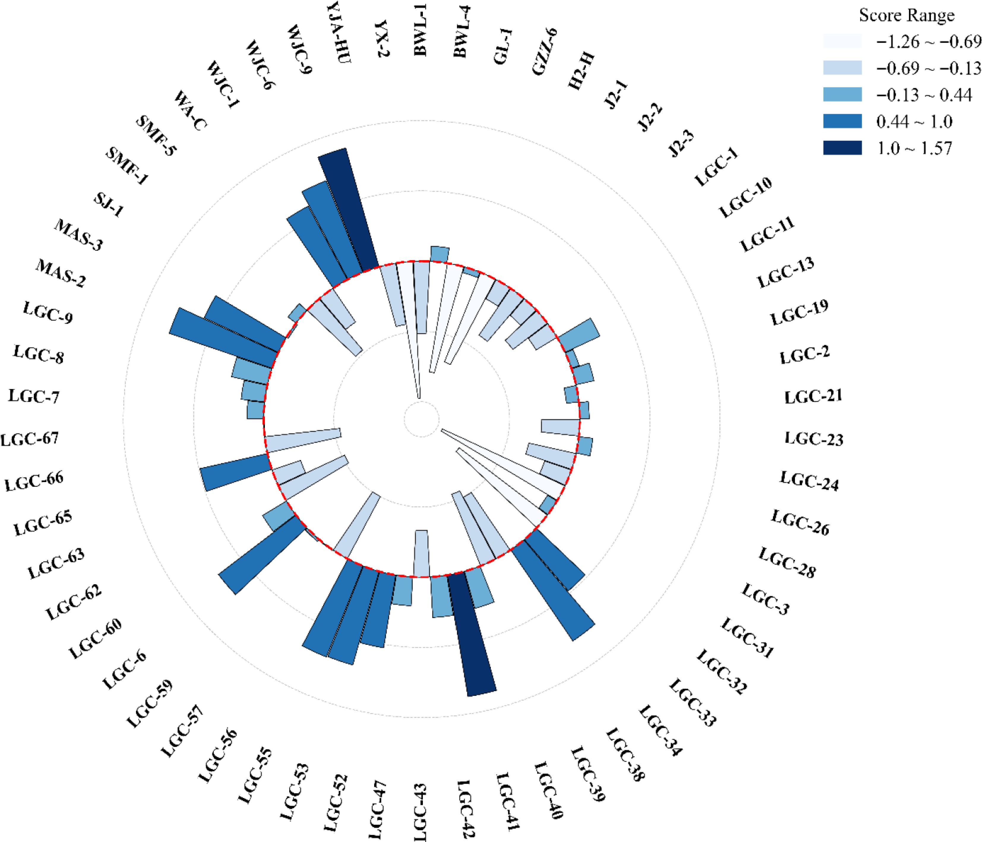
Figure 7.
The F-total value of each Pistacia chinensis clone seedling, indicating the phenotyping differences. The alphabetical prefix (e.g., 'LGC) represents the provenance origin, and the numerical suffix (e.g., '28') identifies the specific clonal lineage within that provenance.
-
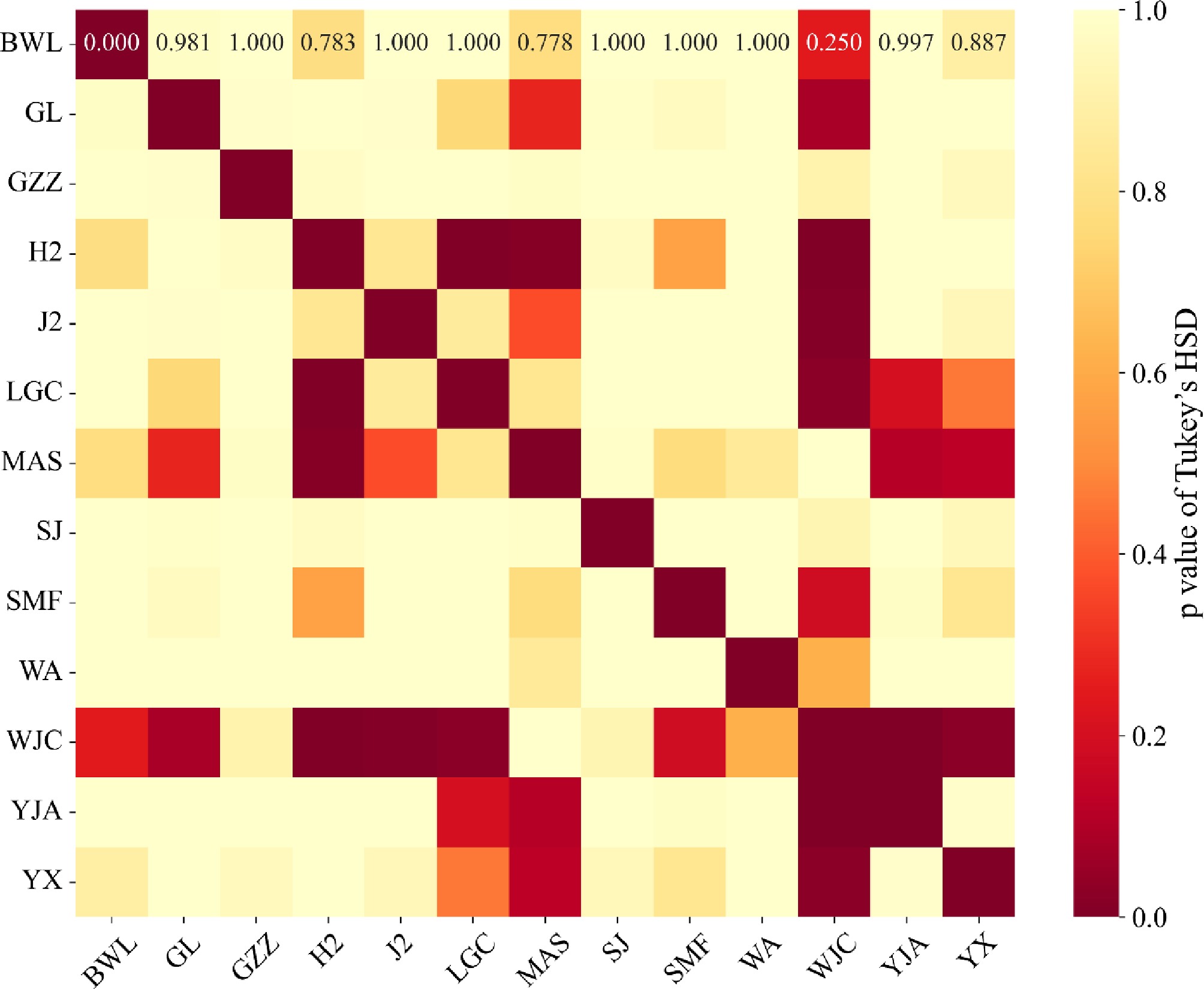
Figure 8.
Heatmap showing the results of pairwise Tukey's HSD tests for differences in F-total among provenances. The color gradient reflects the level of significance, with darker shades indicating lower p-values. Provenances such as WJC and H2 exhibited significant divergence from several others, underscoring provenance-level variation in this trait.
-
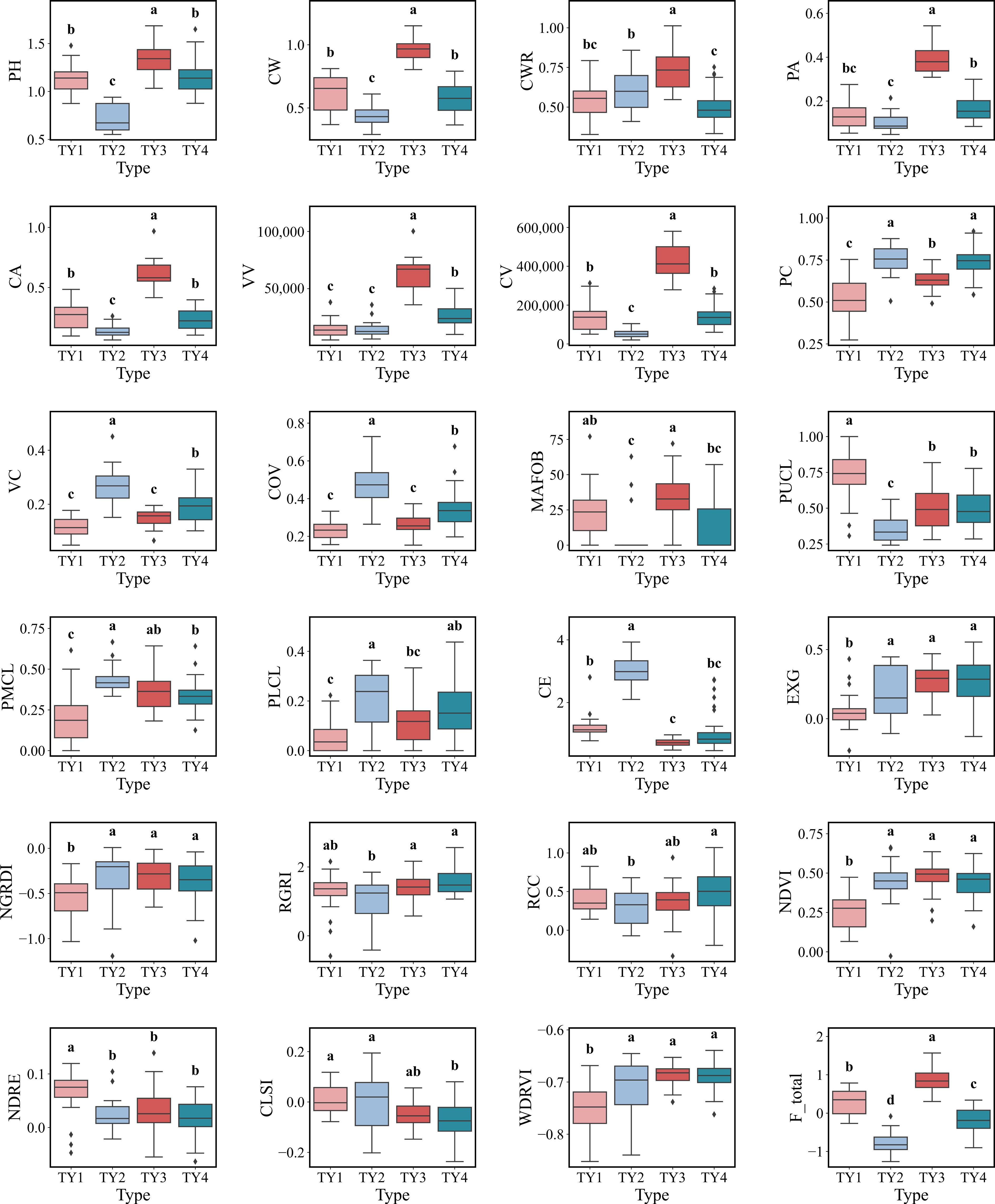
Figure 9.
Box plots of phenotypic traits for the four clusters identified by K-means clustering. The horizontal line within the box indicates the median, boundaries of the box indicate the 25th and 75th percentiles, and whiskers indicate the range. Different lowercase letters (a, b, c, d) above the boxes indicate statistically significant differences among the four clusters based on One-way ANOVA followed by Tukey's HSD test (p < 0.05).
-
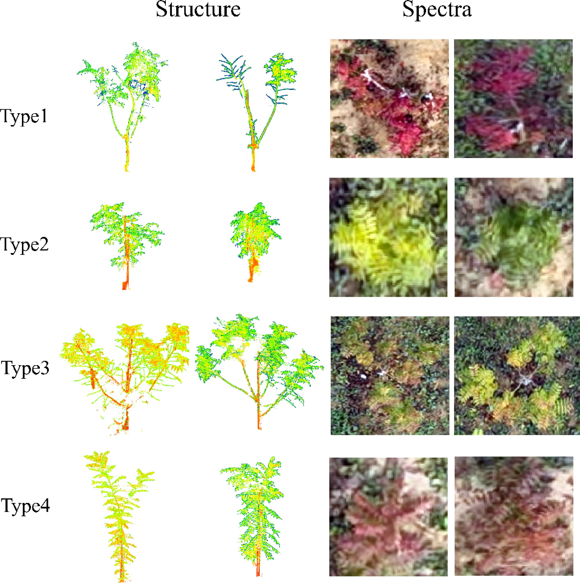
Figure 10.
Two representative individuals were selected from distinct clonal types of P. chinensis to illustrate structural (point cloud) and spectral (RGB imagery from UAV) characteristics, highlighting marked phenotypic differences between types.
-
Traits (unit) Range Mean ± standard deviation Plant height (m) 0.48–1.65 1.14 ± 0.26 Scion diameter (mm) 7.48–30.36 20.05 ± 5.62 Crown width (m) 0.19–1.11 0.62 ± 0.21 Mean angle of first-order branches (°) 16.50–67.83 37.59 ± 11.79 Number of compound leaves (pieces) 6–85 29 ± 14 Table 1.
Overview of the ground-based survey of representative phenotypic traits used in the traditional P. chinensis clonal selection.
-
Types Traits (abbreviation) Definition Ref. Growth traits Plant height (PH) Height of an individual seedling [31] Crown width (CW) Mean crown width in the X and Y directions [31] Crown width ratio (CWR) Ratio of crown width to plant height [31] Maximum crown height (MCH) The height corresponding to the layer with the largest crown width was recorded [31] Morphological traits Projection area (PA) Vertically projected area of the crown of an individual seedling [18] Convex-hull area (CA) Convex hull area of an individual seedling in the XY plane for the vertically-projected point cloud [18] Voxel-based volume (VV) Volume of the voxelized crown of an individual seedling [18] Convex-hull volume (CV) Volume of the convex hull of the crown of an individual seedling [18] Projection compactness (PC) Ratio of projection area to convex-hull area [18] Volume compactness (VC) Ratio of voxel-based volume to convex-hull volume [18] Canopy occupation volume (COV) Ratio of the number of occupied voxels to the total number of voxels [32] Mean of first-order branch angles (MFBA) Mean of the angles between first-order branches and the main stem. [33] Relative leaf abundance Ratio of the number of compound leaves at a specific layer to the total number of those in all layers (LCLP, MCLP UCLP) [33] Architecture complexity Canopy entropy (CE) A metric to simplify forest canopy structural complexity and spatial heterogeneity. [19] Table 2.
Summary of TLS-derived structural traits of Pistacia chinensis seedlings.
-
Sensor Vegetation indices Formula Ref. Multispectral Normalized Difference Vegetation Index (NDVI) $ NDVI=\dfrac{{NIR}_{m}-{R}_{m}}{{NIR}_{m}+{R}_{m}} $ [34] Normalized Difference Red Edge Index (NDRE) $ NDRE=\dfrac{{NIR}_{m}-{RE}_{m}}{{NIR}_{m}+{RE}_{m}} $ [35] Chlorophyll Leaf Senescence Index (CLSI) $ \text{CLSI}=\dfrac{R{E}_{m}-{G}_{m}}{R{E}_{m}+{G}_{m}}-R{E}_{m} $ [36] Weighted Difference Vegetation Index (WDRVI) $ \text{WDRVI}=\dfrac{\alpha \cdot NI{R}_{m}-{R}_{m}}{\alpha \cdot NI{R}_{m}+{R}_{m}} $ [37] RGB Excess Green Index (EXG) $ \text{EXG}=2\times {G}_{v}-{R}_{v}-{B}_{v} $ [34] Normalized Green-Red Difference Index (NGRDI) $ \text{NGRDI}=\dfrac{{G}_{v}-{R}_{v}}{{G}_{v}+{R}_{v}} $ [38] Red-Green Ratio Index (RGRI) $ \text{RGRI}=\dfrac{{R}_{v}}{{G}_{v}} $ [39] Red Chromatic Coordinate (RCC) $ \text{RCC}=\dfrac{{R}_{v}}{{R}_{v}+{G}_{v}+{B}_{v}} $ [34] Note that the indices requiring the blue band were computed using the corresponding RGB imagery. The subscripts $ m $ $ v $ Table 3.
Summary of vegetation indices calculated based on multispectral or RGB imagery.
-
Traits Mean SD Min Max CV % PH 1.11 0.25 0.55 1.69 22.71 CW 0.64 0.21 0.29 1.15 32.78 CWR 0.58 0.15 0.33 1.01 25.06 PA 0.19 0.12 0.05 0.54 60.48 CA 0.30 0.19 0.06 0.97 64.21 VV 29,265.82 20,693.74 5,224.00 100,144.00 70.71 CV 185,124.08 144,665.50 20,731.35 580,001.78 78.15 PC 0.67 0.13 0.27 0.92 19.01 VC 0.18 0.08 0.05 0.45 40.80 COV 0.33 0.12 0.15 0.73 35.44 MFBA 18.22 20.51 0.00 77.09 112.61 LCLP 0.53 0.19 0.24 1.00 35.85 MCLP 0.33 0.14 0.00 0.67 42.05 UCLP 0.14 0.11 0.00 0.44 80.25 CE 1.40 0.94 0.47 3.93 67.12 EXG 0.21 0.17 −0.23 0.55 80.93 NGRDI −0.39 0.24 −1.19 0.01 62.64 RGRI 1.36 0.51 −0.59 2.56 37.65 RCC 0.41 0.26 −0.34 1.07 63.36 NDVI 0.41 0.14 −0.03 0.66 34.14 NDRE 0.03 0.04 −0.06 0.14 117.42 CLSI −0.03 0.08 −0.24 0.19 238.25 WDRVI −0.71 0.04 −0.85 −0.64 6.12 Note: CV (%) = SD/mean × 100%. Table 4.
Descriptive statistics of TLS-derived structural traits and UAV-derived spectral traits across the entire seedling population.
Figures
(10)
Tables
(4)