-
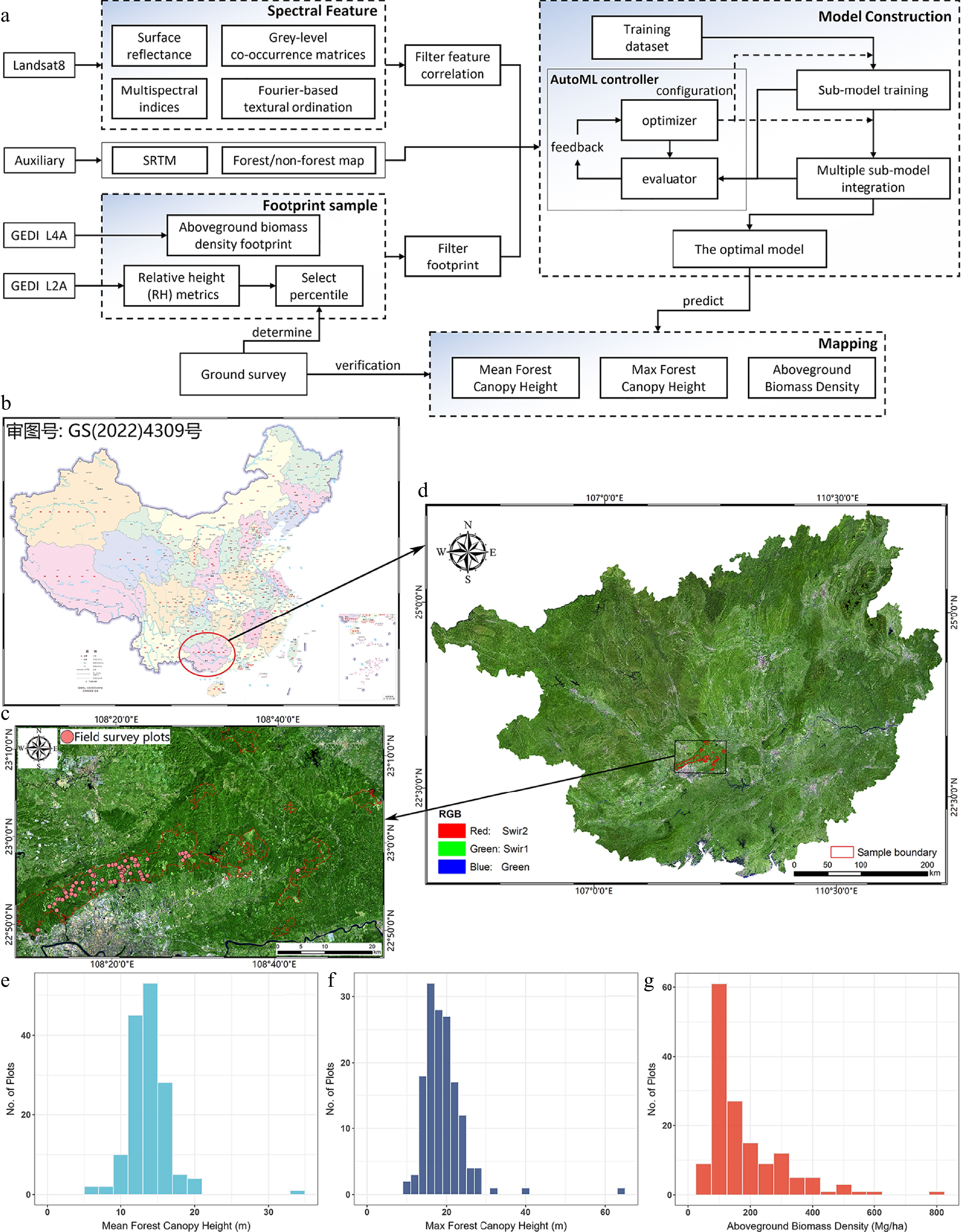
Figure 1.
(a) Flowchart of proposed methods. The study area is located in Guangxi Province in China. The ground survey area is located in (b) Gaofeng forestry, with (c) red boundary and pink field survey plots. (d) The overview of the study area. The distribution of (e) mean FCH, (f) max FCH, and (g) AGBD.
-
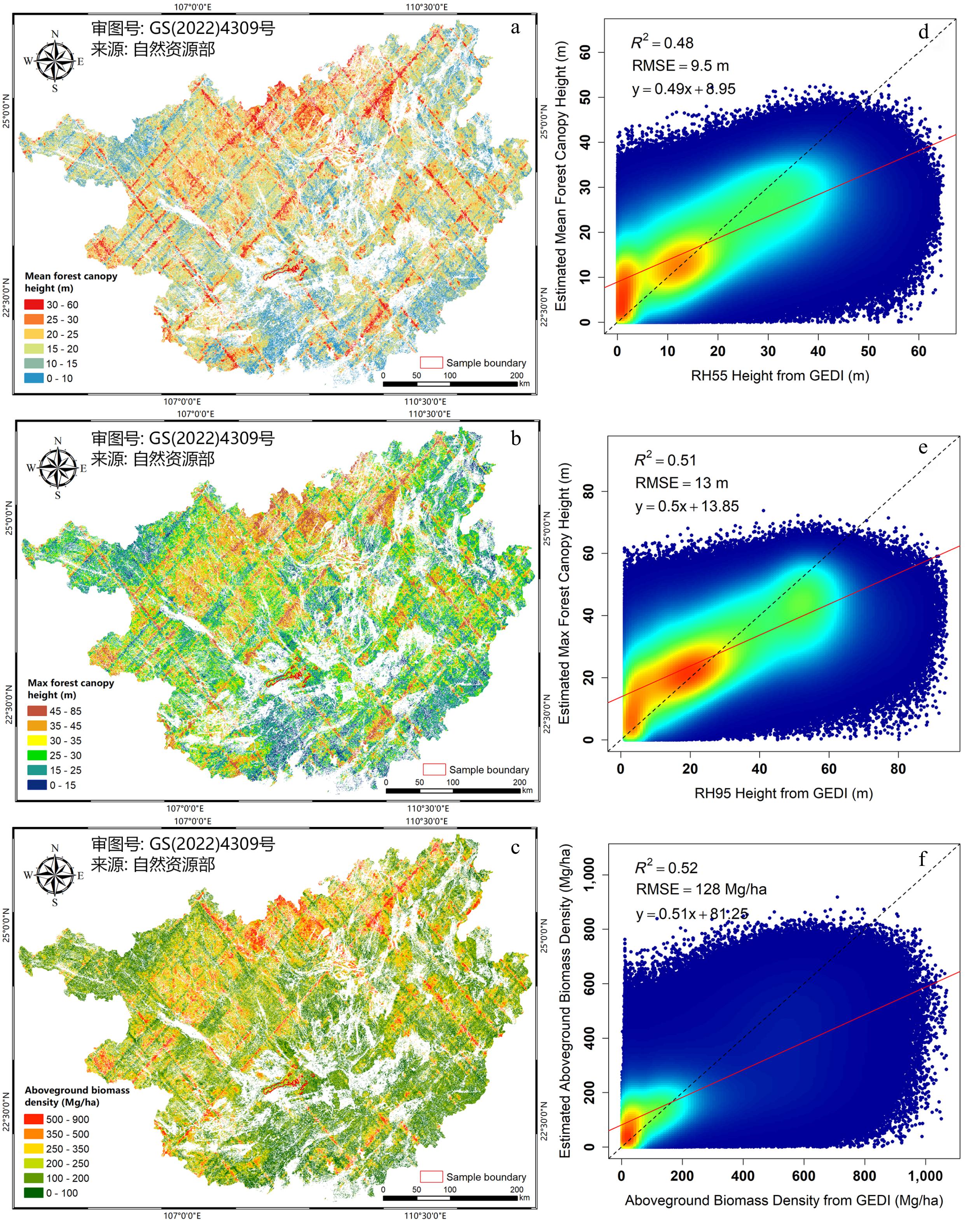
Figure 2.
The mapping results of the (a) mean FCH, (b) max FCH, and (c) AGBD. (d)–(f) The scatter plots of the corresponding results of test sets, respectively.
-
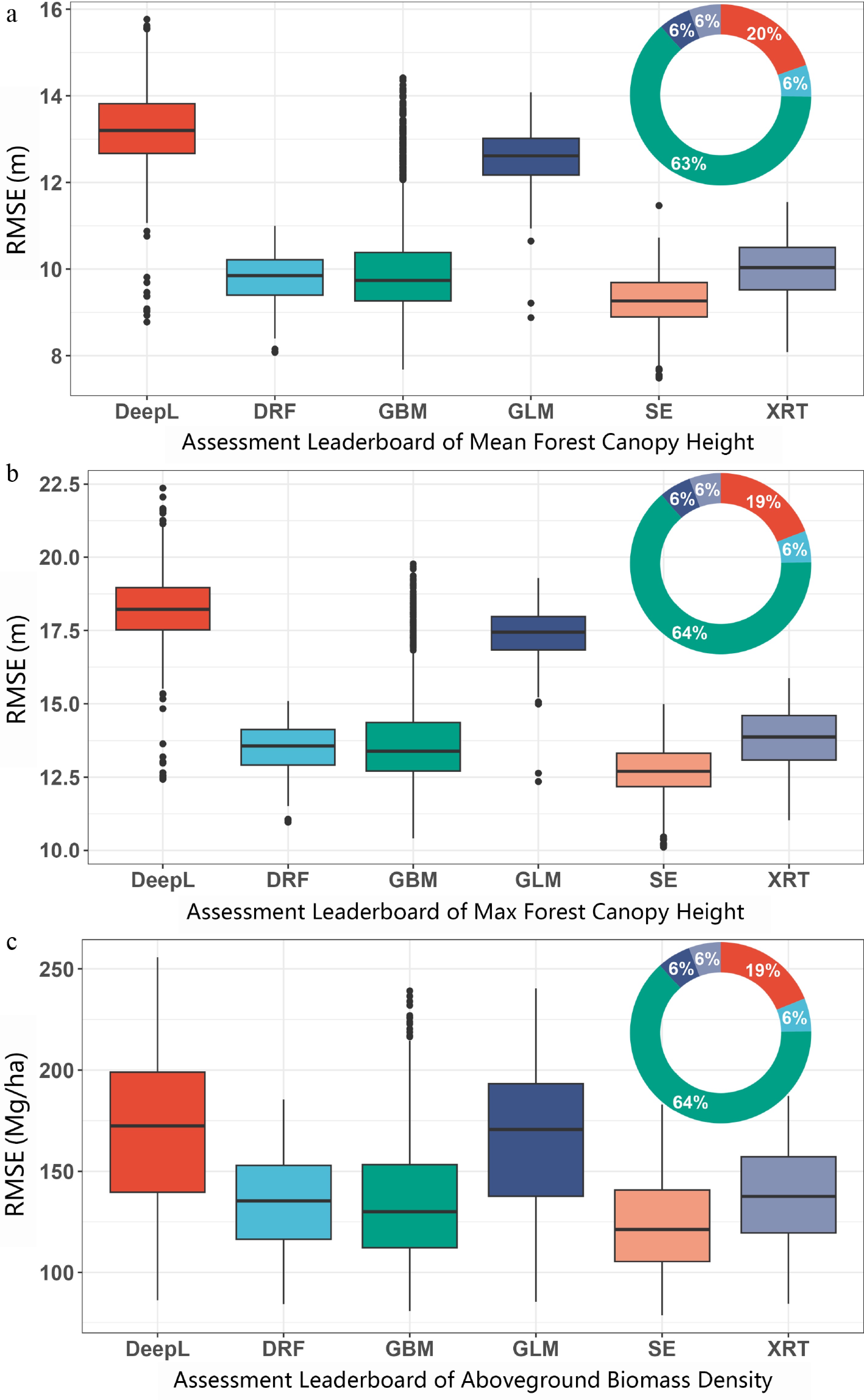
Figure 3.
The RMSE of models trained by AutoML in (a) mean FCH, (b) max FCH, and (c) AGBD mapping. The frequency percentage in the pie chart is of the best performing SE model in sub-model combination from the model building process.
-
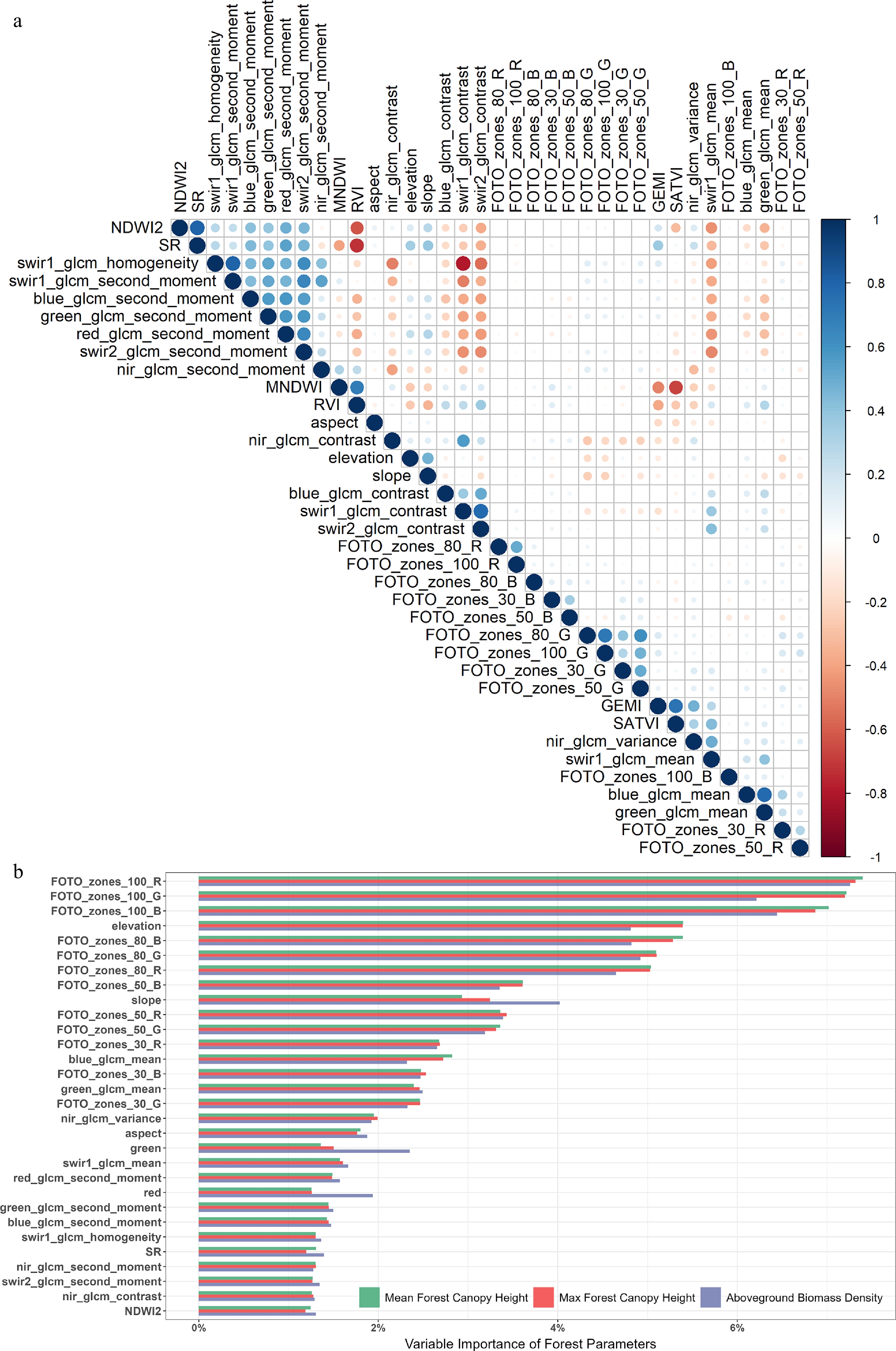
Figure 4.
(a) Linear relationship plot between each feature. Only the results of the filtered features are shown here. (b) The variable importance of regression models was calculated in mean FCH, max FCH, and AGBD mappings within the whole Guangxi province. Variables have been sorted according to their importance, and each variable was defined in Table 2. Only the top 30 features are shown here.
-
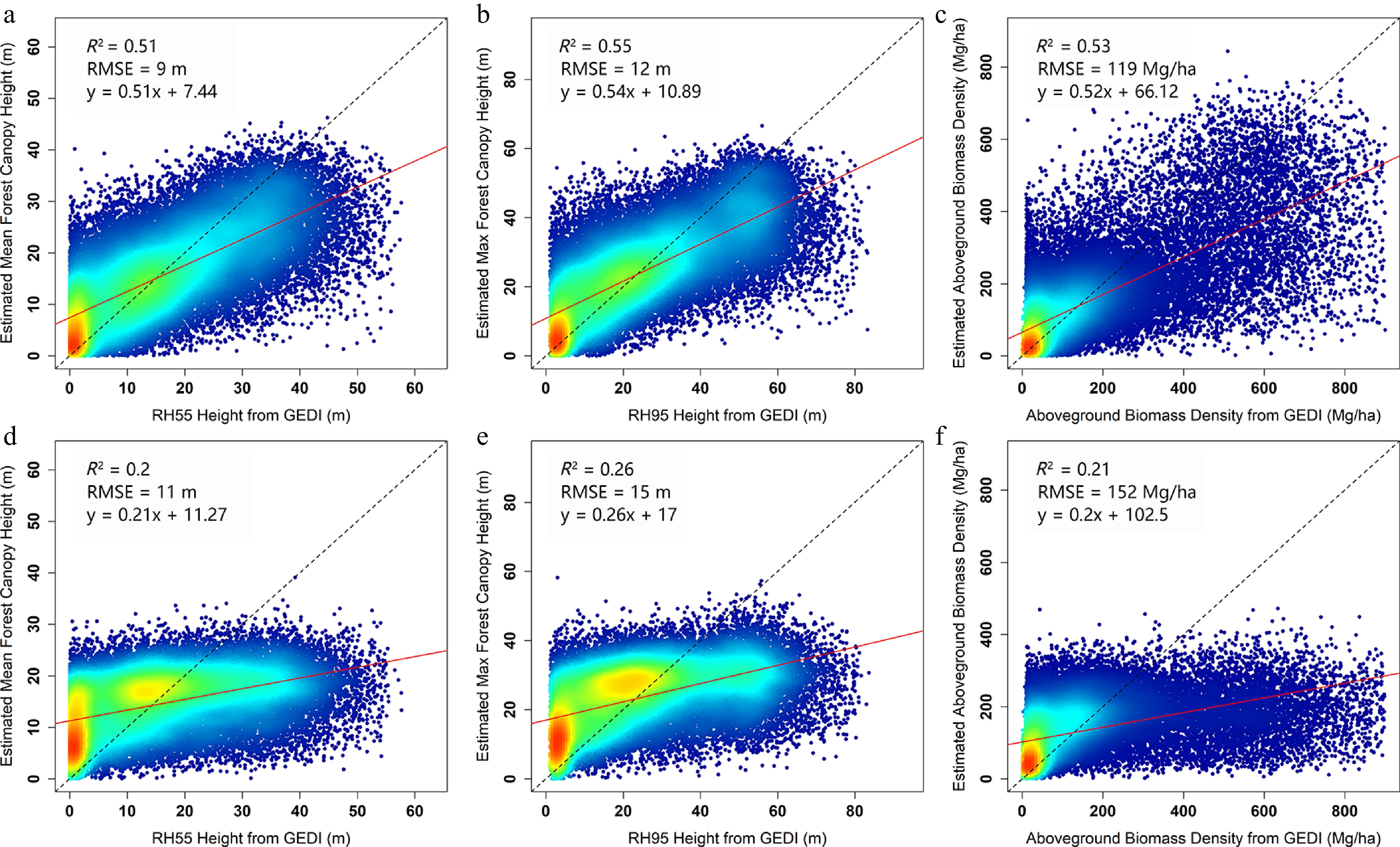
Figure 5.
Scatter plots measuring the enhancement of FOTO features on the regression ability of model training. (a) and (d) show the scatter plots of mean FCH regression model training after adding FOTO features for sample areas respectively. (b) and (e) show the scatter plots of max FCH regression model training after adding FOTO features for sample areas respectively. (c) and (f) show the scatter plots of AGBD regression model training after adding FOTO features for sample areas.
-
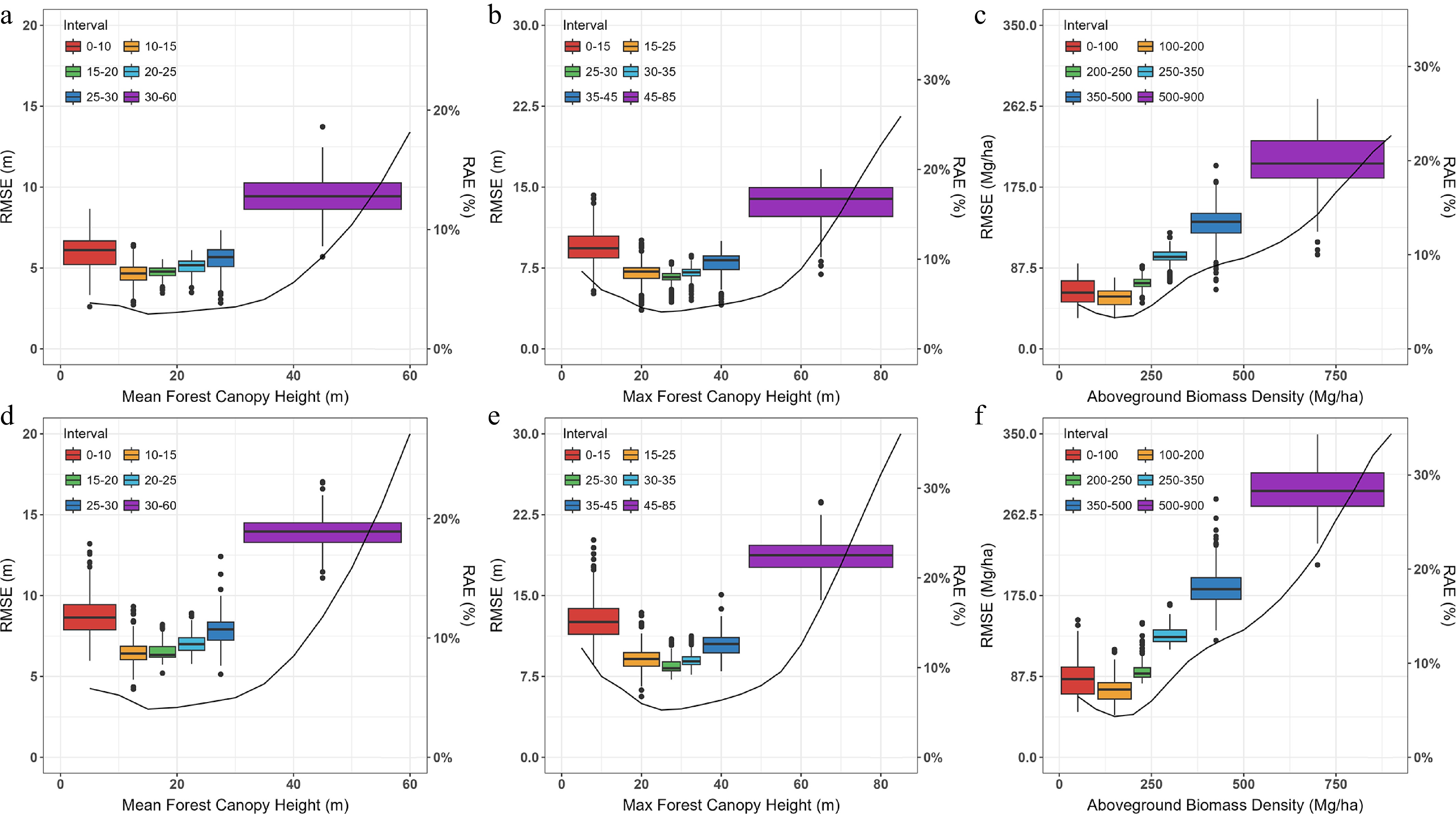
Figure 6.
Uncertainty within, and between estimation intervals for three forest parameters ([a] and [d] for mean FCH, [b] and [e] for max FCH, [c] and [f] for AGBD). (a)–(c), and (d)–(f) show the estimation accuracy of the training sets and test sets in each interval, respectively.
-
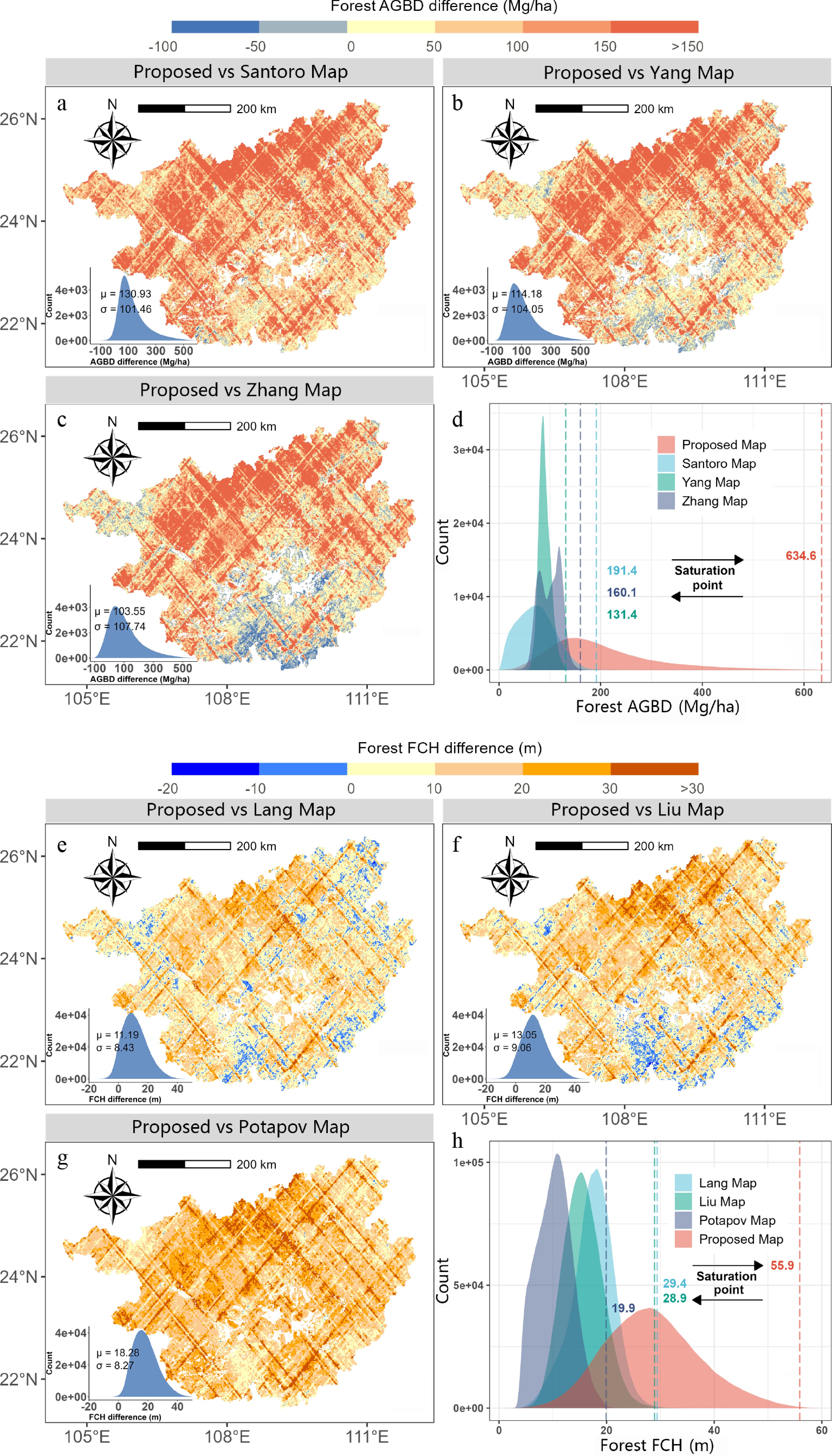
Figure 7.
(a)–(c) Differences between the proposed AGBD mapping result and other products. (d) The AGBD distribution of each product. (e)–(g) Differences between proposed max FCH mapping result and other products. (h) Max FCH distribution of each product.
-
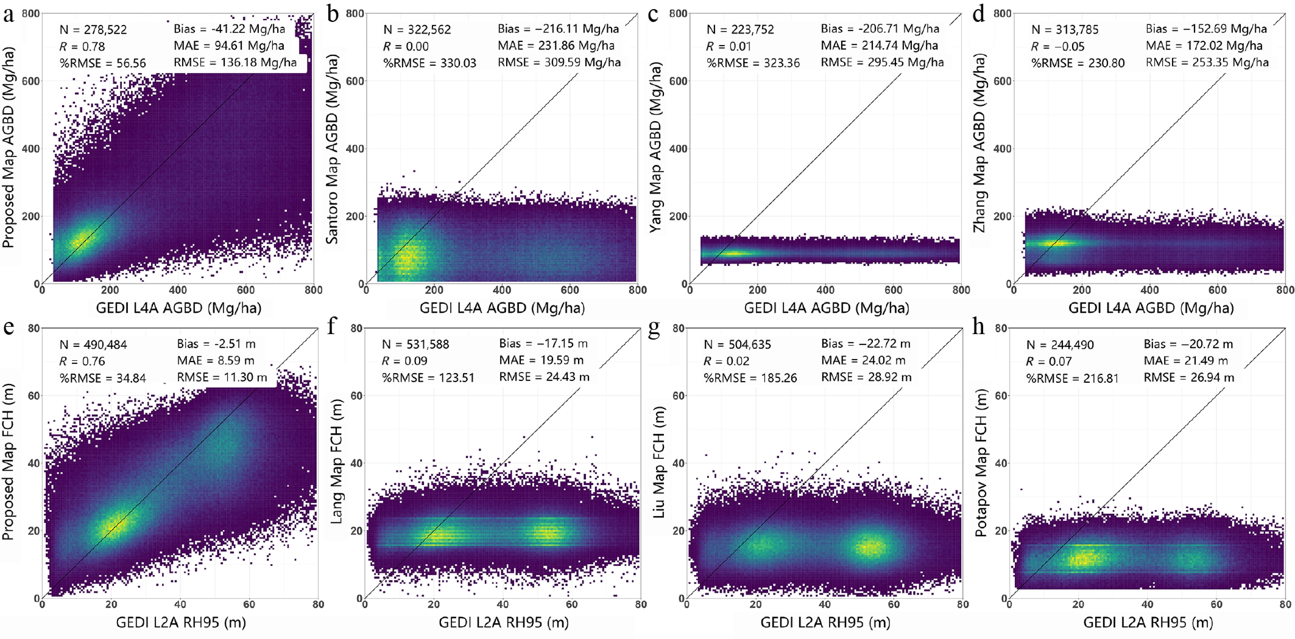
Figure 8.
(a)–(d) Scatter plots between the GEDI L4A footprint product and the four AGBD map types. (e)–(h) Scatter plots between the GEDI L2A RH95 height footprint products and the four max FCH maps.
-
Step Process/logic Description 1 for $ \tau $ $ \mathrm{T} $ T-layer stacking iteration. 2 for $ \upsilon $ $ \mathrm{N} $ N-repeated bagging for stability. 3 Randomly partition data (X, Y) into K segments $ {\left\{{\mathrm{X}}^{\lambda },{\mathrm{Y}}^{\lambda }\right\}}_{\lambda \in \mathrm{K}} $ K-fold random data partition. 4 for $ \lambda $ $ \mathrm{K} $ K-fold bagging loop. 5 for each type $ \rho $ $ \mathrm{P} $ Train each base model type ρ on training folds. 6 Train a ρ-type model on $ \left\{{\mathrm{X}}^{\lambda },{\mathrm{Y}}^{\lambda }\right\} $ $ {\hat{Y}}_{\rho ,\lambda }^{\upsilon} $ Generate out-of-fold (OOF) predictions. 7 Compute average OOF predictions $ {\hat{Y}}_{\rho ,\tau }={\left\{\dfrac{1}{N}{\sum }_{\upsilon }\hat{Y}_{\rho ,\lambda }^{\upsilon }\right\}}_{\lambda \in \mathrm{K}} $ Average OOF predictions across N repetitions. 8 G ← aggregate(X, $ {\left\{{\hat{Y}}_{\rho ,\tau }\right\}}_{\rho \in \mathrm{P},\tau \in \mathrm{T}} $ Train meta-learner with aggregated predictions. 9 $ \hat{Y} $ Generate final predictions. The text in bold indicates variables for which values can be entered during the modeling process. Symbols: X: feature set; Y: target set; P: finite set of base model types (e.g., DRF, GBM, GLM, etc.); T: number of stacking layers; N: number of bagging repetitions; K: number of cross-validation folds. Table 1.
The key steps of the AutoML algorithm used in this paper.
-
Features Description Bands in calculation Source Spectral Surface reflectance Band2–band7 Landsat8 CTVI Corrected Transformed Vegetation Index Red, nir [31] DVI Difference Vegetation Index Red, nir [32] EVI Enhanced Vegetation Index Red, nir, blue [33] EVI2 Two-band Enhanced Vegetation Index Red, nir [34] GEMI Global Environmental Monitoring Index Red, nir [35] GNDVI Green Normalised Difference Vegetation Index Green, nir [36] KNDVI Kernel Normalised Difference Vegetation Index Red, nir [37] MNDWI Modified Normalised Difference Water Index Green, swir1 [38] MSAVI Modified Soil Adjusted Vegetation Index Red, nir [39] MSAVI2 Modified Soil Adjusted Vegetation Index 2 Red, nir [39] NBRI Normalised Burn Ratio Index Nir, swir2 [40] NDVI Normalised Difference Vegetation Index Red, nir [41] NDWI Normalised Difference Water Index Green, nir [42] NDWI2 Normalised Difference Water Index 2 Nir, swir1 [43] NRVI Normalised Ratio Vegetation Index Red, nir [44] RVI Ratio Vegetation Index Red, nir [45] SATVI Soil Adjusted Total Vegetation Index Red, swir1,
swir2[46] SAVI Soil Adjusted Vegetation Index Red, nir [47] SLAVI Specific Leaf Area Vegetation Index Red, nir, swir1 [48] SR Simple Ratio Vegetation Index Red, nir [49] TTVI Thiam's Transformed Vegetation Index Red, nir [50] TVI Transformed Vegetation Index Red, nir [51] WDVI Weighted Difference Vegetation Index Red, nir [32] Elevation NASA SRTM Digital Elevation 30m — NASA/USGS Slope Slope from SRTM Digital Elevation — Google Earth Engine Aspect Aspect from SRTM Digital Elevation — Google Earth Engine GLCM Grey Level Co-Occurrence matrices Band2–band7 [52] FOTO Fourier-based Textural Ordination Nir [25] Table 2.
Landsat8 features and auxiliary datasets including spectral indices, texture, spectral transform, and terrain information.
-
RH percentile RH 45 RH50 RH55 RH60 RH65 RH70 RH75 RH80 RH85 RH90 RH95 RH 99 RH100 Unit Mean FCH 5.99 5.78 5.63 6.12 6.85 7.69 8.31 9.29 10.08 11.35 12.13 13.30 14.05 m Max FCH 10.15 9.70 9.46 9.01 8.31 8.35 8.29 8.61 8.69 7.88 7.21 7.49 8.53 The values in bold are the metrics used in this method. Table 3.
Results of determining the correspondence between GEDI LiDAR height response and forest parameters based on ground survey plots, showing RMSE difference.
-
Parameters Mean Unit RMSE RAE (%) Bias Mean FCH 13.70 m 5.63 41.0 −2.67 Max FCH 18.86 m 7.21 38.2 −2.99 AGBD 153.19 Mg/ha 81.00 52.8 −36.50 Table 4.
Assessing the accuracy of forest parameter mapping using sample plots within Gaofeng forestry.
-
Type Source Resolution (m) Date Materials AGBD [5] 100 2020 Sentinel-1, ASAR, ALOS-1/2, Auxiliary (GEDI, ICESat-2) [55] 30 2019 Forestry survey fields, Features (FCH, Terrain, Climate and Soil) [56] 30 2021 Forestry survey fields, Landsat, FCH max FCH [57] 10 2020 GEDI, Sentinel-2 [58] 30 2019 GEDI, ICESat-2, Sentinel-2 [16] 30 2019 GEDI, Landsat Table 5.
Major information and sources for the large-scale forest parameter mapping products selected in this paper.
-
Type Mapping source RMSE (Mg/ha) RAE (%) Bias (Mg/ha) AGBD Proposed mapping 81.00 52.8 −36.50 [5] 127.88 83.5 −111.16 [55] 120.68 78.8 −109.72 [56] 99.96 65.3 −75.59 Type Mapping source RMSE (m) RAE (%) Bias (m) max FCH Proposed mapping 7.21 38.2 −2.99 [57] 9.69 51.4 −4.45 [58] 9.27 49.2 −9.42 [16] 11.97 63.5 −9.80 Table 6.
Assessing the accuracy of products using sample plots within Gaofeng forestry.
Figures
(8)
Tables
(6)