-
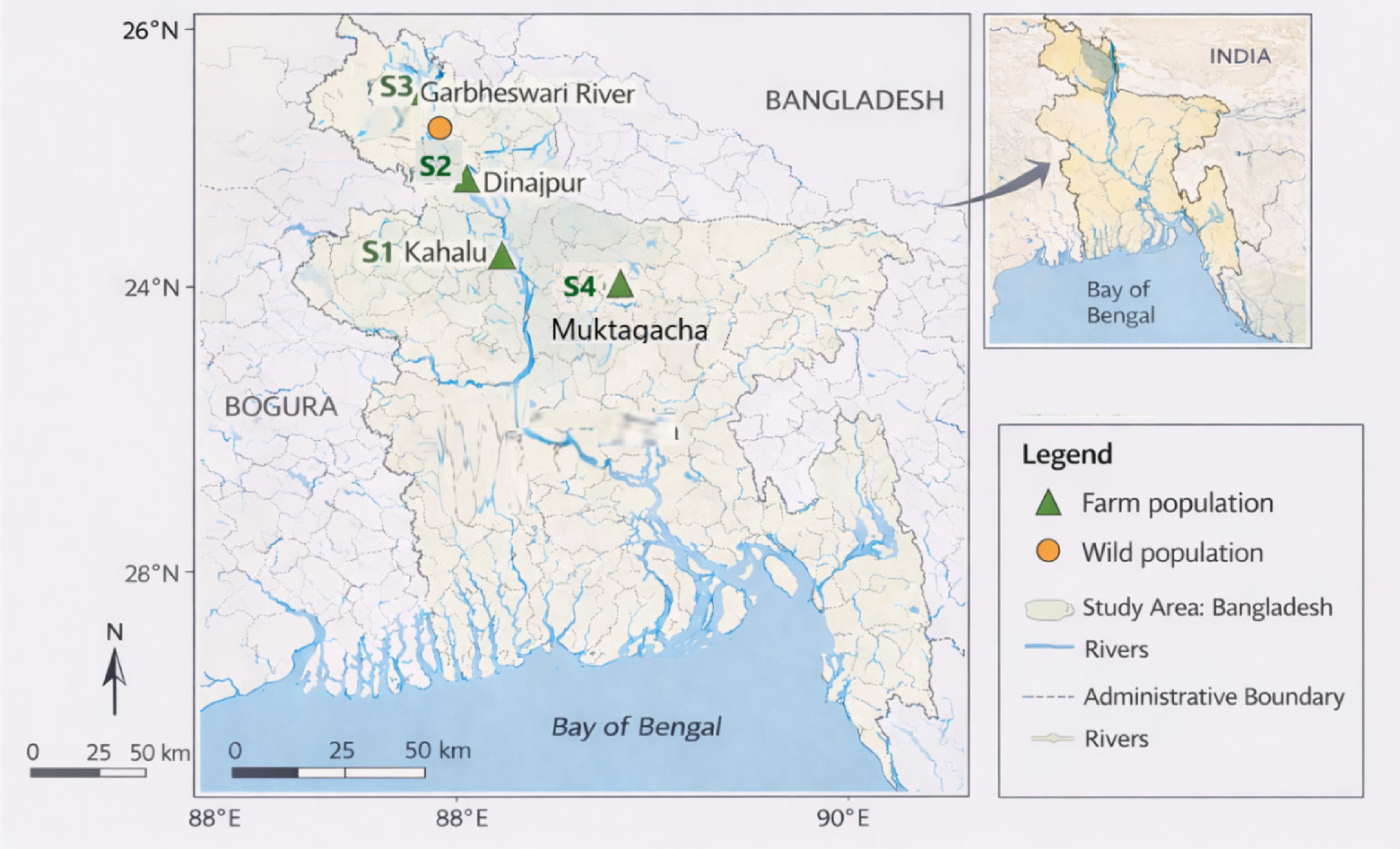
Figure 1.
Sampling locations of farmed and wild populations of Heteropneustes fossilis in Bangladesh. Source: Created by the authors using sampling coordinates and GIS datasets from the Global Map Initiative and LGED, Bangladesh.
-
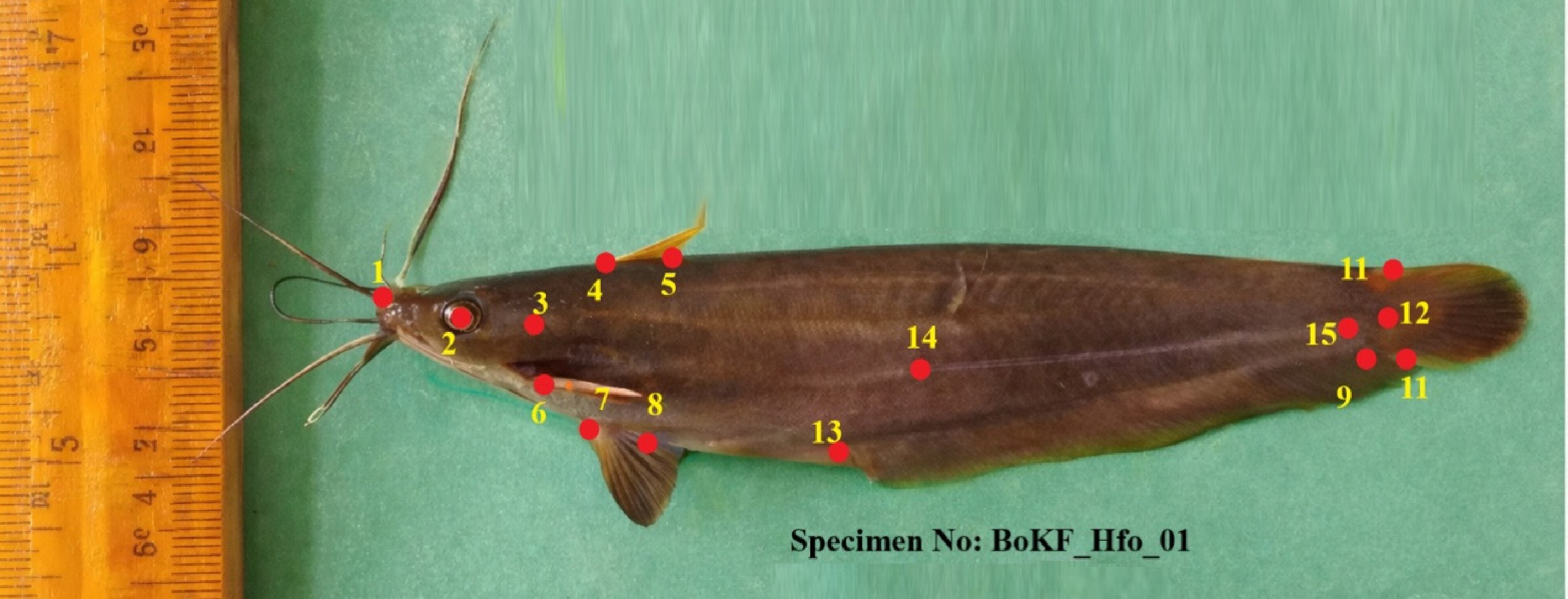
Figure 2.
Digital image acquisition and geometric morphometric landmark configuration of H. fossilis: Landmarks: 1, tip of snout (anterior-most point of upper jaw); 2, center of eye; 3, posterior margin of operculum; 4, origin of dorsal fin; 5, end of dorsal fin base; 6, origin of pectoral fin; 7, origin of pelvic fin; 8, origin of anal fin; 9, end of anal fin base; 10, dorsal insertion of caudal fin; 11, ventral insertion of caudal fin; 12, center of caudal fin (hypural plate tip); 13, point above anus between pelvic and anal fins; 14, mid-body point along lateral line; 15, posterior termination of lateral line or posterior belly margin.
-
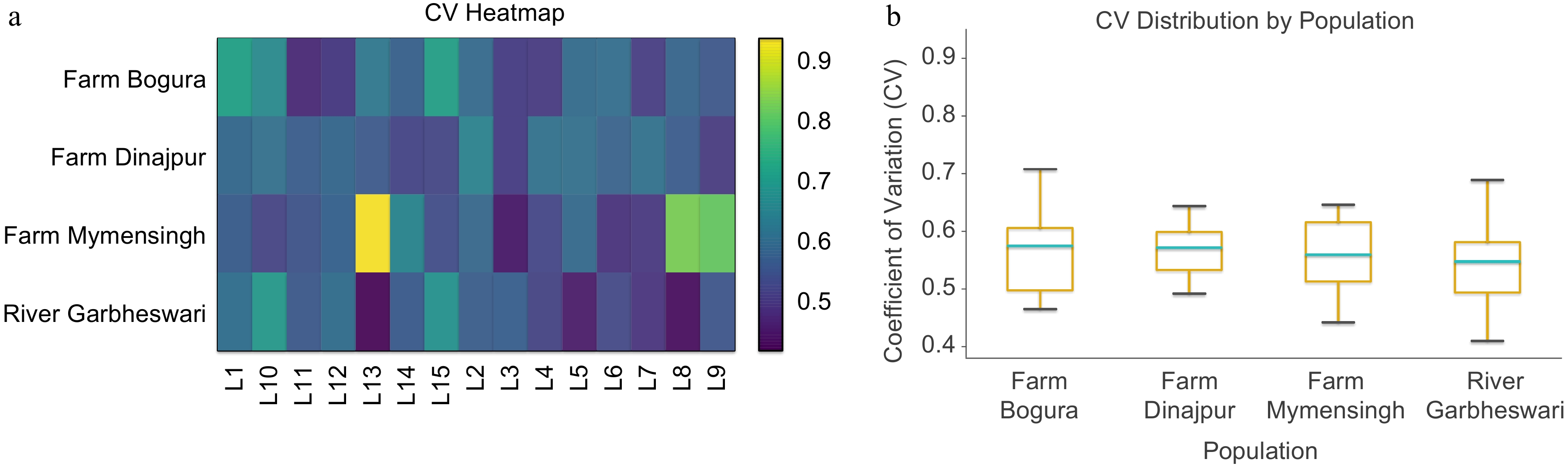
Figure 3.
(a) Heatmap, and (b) boxplot showing CV-based morphological variability in 15 landmarks among four H. fossilis populations. Both visualizations reveal clear population-level differences, with river fish exhibiting greater trait variation than farmed stocks.
-
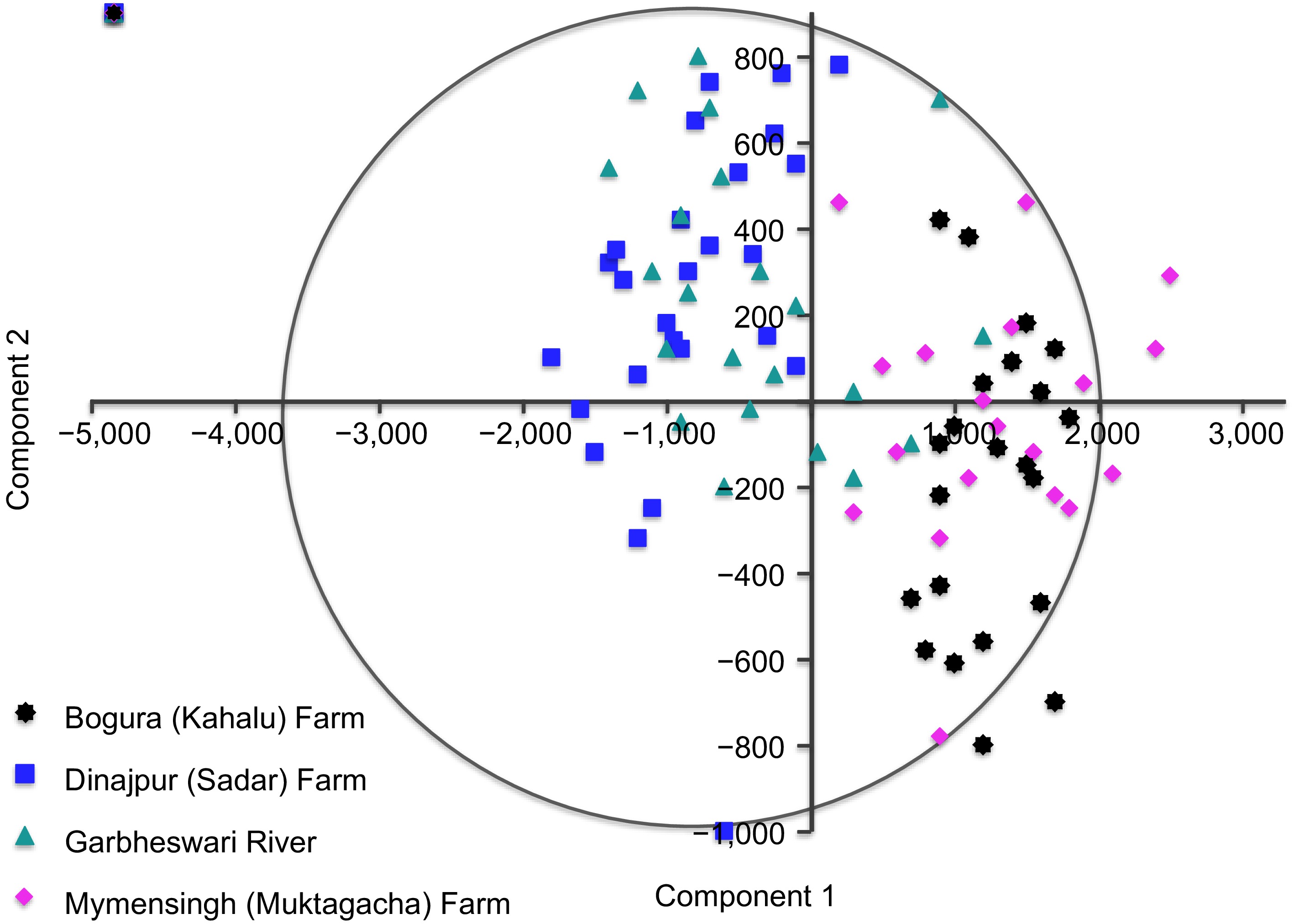
Figure 4.
Principal Component Analysis (PCA) scatter plot of relative warp scores showing morphological variation and differentiation among four Heteropneustes fossilis stocks in Bangladesh.
-
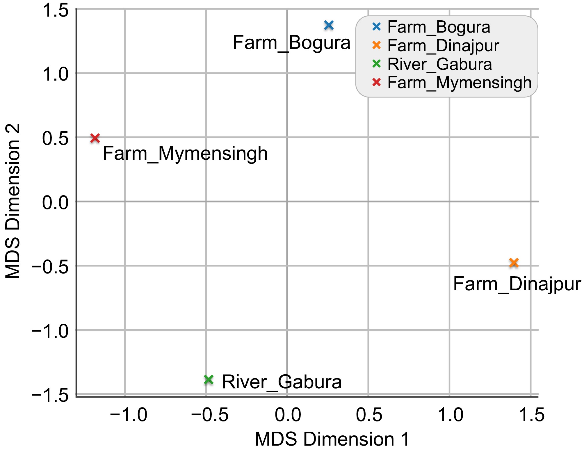
Figure 5.
Multidimensional scaling (MDS) plot of H. fossilis populations based on mahalanobis distances.
-
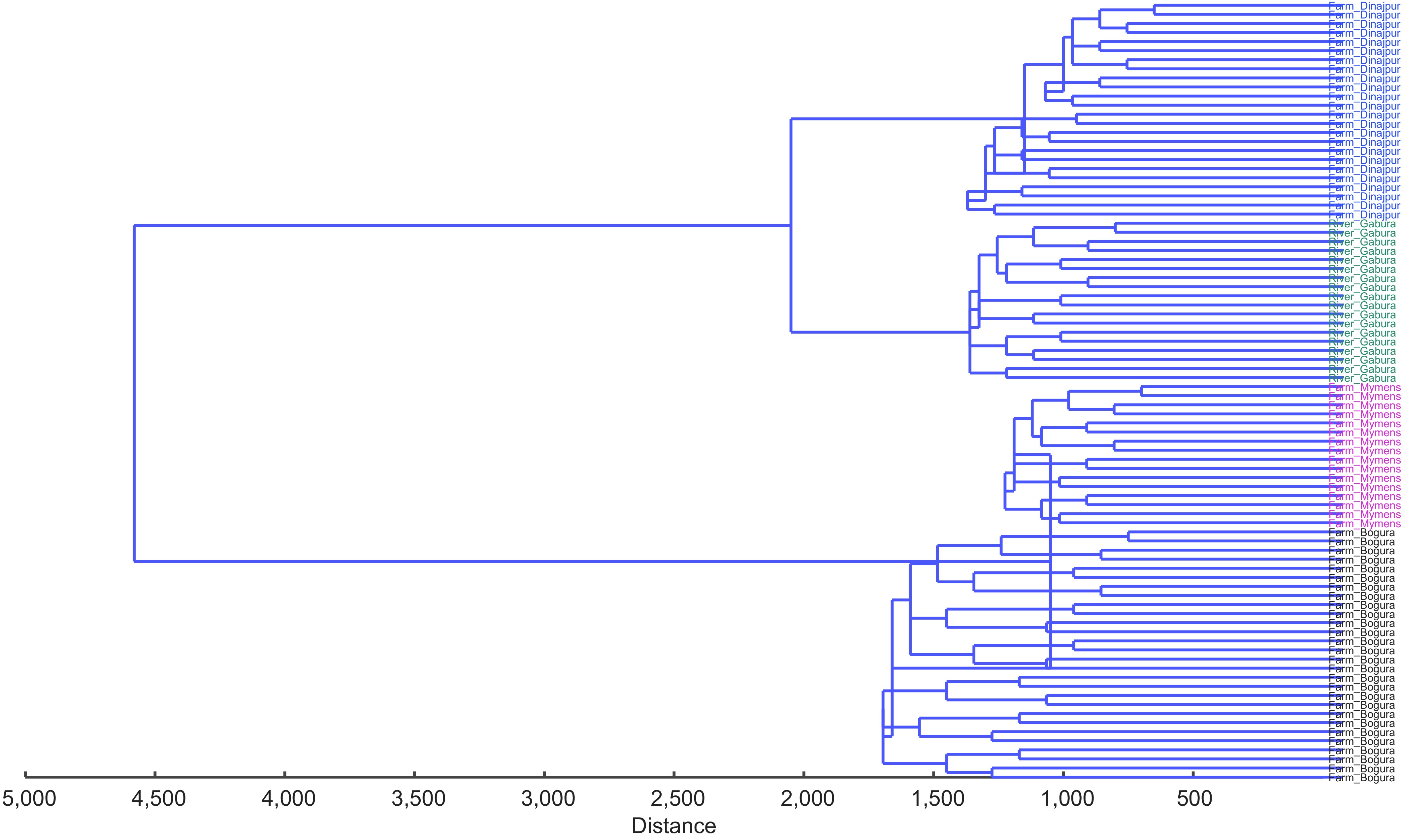
Figure 6.
The UPGMA dendogram clustering three H. fossilis populations collected from the Farm Bogura (Kahalu) (black) Farm Dinajpur (Sadar) (blue), Farm-Mymensingh (Muktagacha) (pink) and River (green).
-
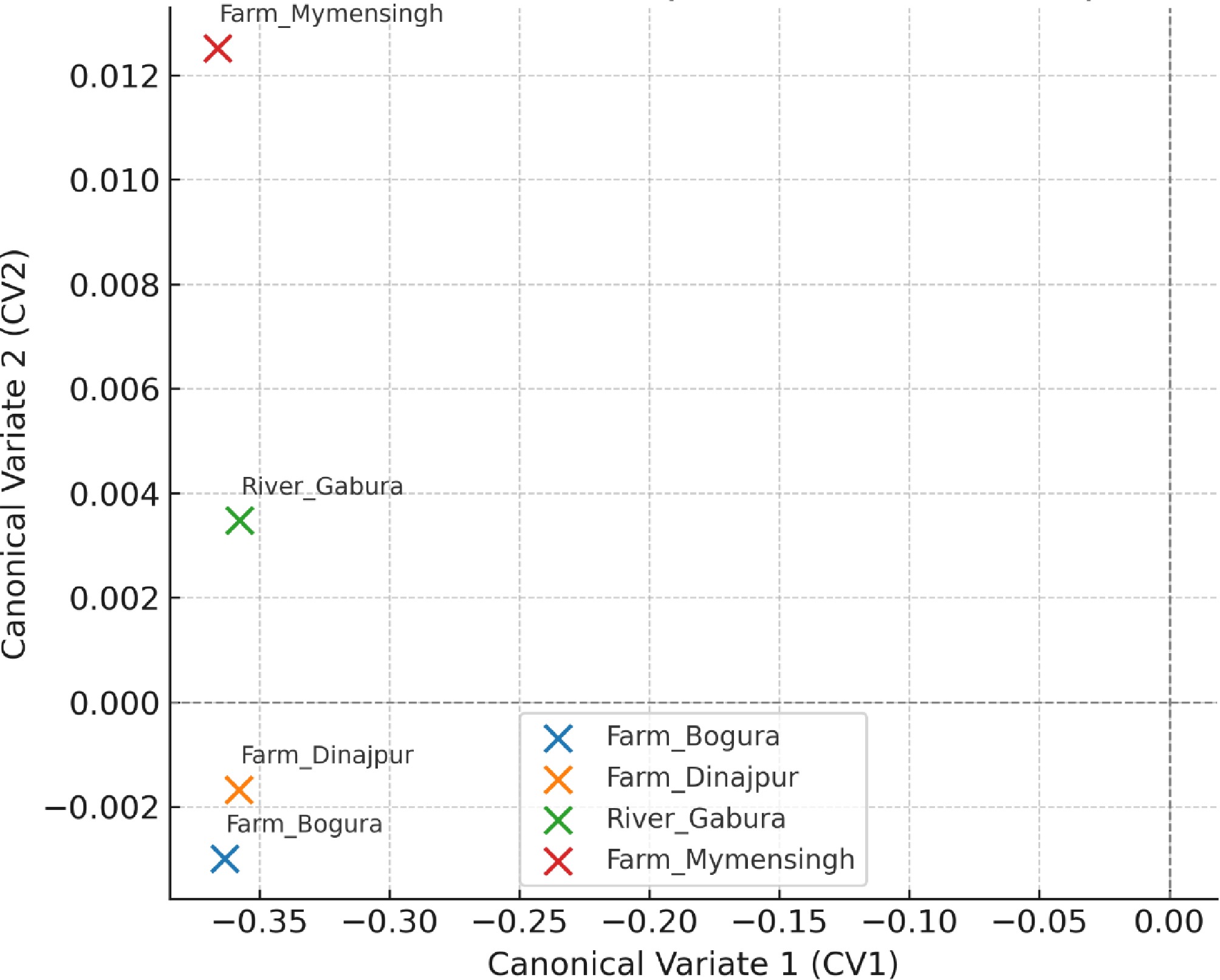
Figure 7.
Discriminant Function Analysis (DFA) scatter plot of H. fossilis populations based on shape variables.
-
Serial no. Sampling site Latitude and longitude Specimens number 01 Bogura (Kahalu) farm 24.835225302963003 N; 89.26866417906673 E 30 02 Dinajpur (Sadar) farm 25.515162905939953 N; 88.61912356122421 E 30 03 Garbheswari River 25.725668118276733 N; 88.68229494916801 E 30 04 Mymensingh (Muktagacha) farm 24.78422504560068 N; 90.25608648359352 E 24 Table 1.
Sampling sites and geographical coordinates of H. fossilis specimens.
-
PC No. Eigenvalue % Variance PC No. Eigenvalue % Variance 1 2.07E+06 88.181 16 180.234 0.007673 2 144,057 6.1326 17 153.718 0.006544 3 79,461.1 3.3827 18 83.192 0.003542 4 34,966.6 1.4885 19 79.7855 0.003397 5 8,666.58 0.36894 20 61.684 0.002626 6 3,730.02 0.15879 21 55.4008 0.002358 7 1,516.44 0.064556 22 53.8798 0.002294 8 1,163.35 0.049525 23 39.1666 0.001667 9 946.928 0.040311 24 34.6372 0.001475 10 612.178 0.026061 25 25.2069 0.001073 11 469.194 0.019974 26 20.2494 0.000862 12 403.822 0.017191 27 18.6412 0.000794 13 300.099 0.012775 28 10.2491 0.000436 14 272.858 0.011616 29 5.17376 0.00022 15 250.168 0.01065 30 4.77664 0.000203 Table 2.
The eigenvalue and percentage variation of four stocks of H. fossilis based on relative wrap analyses.
-
Population pair Pop1 Pop2 Mahalanobis 1 Farm Bogura (Kahalu) Farm Dinajpur 2.476834 2 Farm Bogura (Kahalu) River Garbheswari 2.442656 3 Farm Bogura (Kahalu) Farm Mymensingh 2.005870 4 Farm Dinajpur (Sadar) River Garbheswari 2.328262 5 Farm Dinajpur (Sadar) Farm Mymensingh 2.347969 6 River Garbheswari Farm Mymensingh 2.333033 Table 3.
Pairwise mahalanobis distances between H. fossilis populations.
-
Populations Farm Bogura Farm Dinajpur River Garbheswari Farm Mymensingh Farm Bogura (Kahalu) 24 0 0 6 Farm Dinajpur (Sadar) 0 26 3 1 Farm Mymensingh (Muktagacha) 6 0 1 17 River Garbheswari 0 0 29 1 Table 4.
Classification matrix from Discriminant Function Analysis (DFA) for H. fossilis populations.
-
Canonical function Eigenvalue Canonical correlation (r) Interpretation Can1 2.455 0.844 Very strong group separation Can2 0.261 0.455 Moderate secondary separation Can3 0.090 0.287 Weak additional separation Table 5.
Canonical functions derived from canonical discriminant analysis of four H. fossilis populations.
-
Principal component Can1 Can2 Can3 PC1 0.21 0.08 0.05 PC2 0.74 0.11 0.09 PC3 0.18 0.62 0.14 PC4 0.69 0.16 0.12 PC5 0.12 0.19 0.58 PC6 0.65 0.21 0.51 PC7 0.14 0.57 0.17 PC8 0.09 0.13 0.11 PC9 0.07 0.09 0.08 PC10 0.05 0.06 0.04 Values represent standardized canonical coefficients; higher absolute values (bold) indicate stronger contributions of principal components to the respective canonical functions. Table 6.
Standardized canonical coefficients showing the contributions of principal component scores (PC1–PC10) to the three canonical discriminant functions (Can1–Can3) in the analysis of four H. fossilis populations.
Figures
(7)
Tables
(6)