-
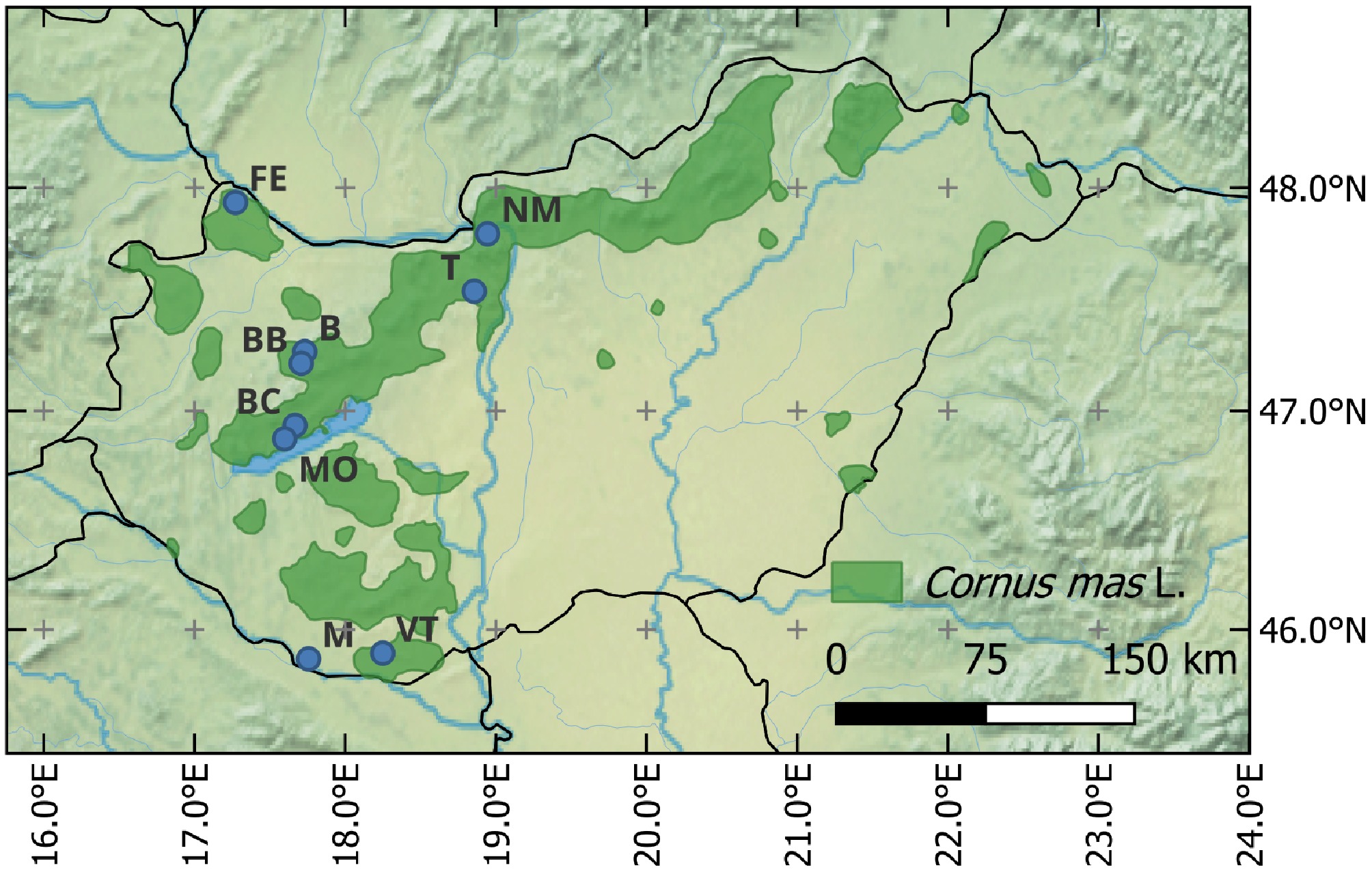
Figure 1.
Sampling sites of Cornus mas in Hungary. B, Bakony, Tönkös- hegy; BB, Bakonybél monastry; BC, Balatoncsicsó; FE, Feketeerdő; M, Markóc; MO, Monoszló; NM, Nagymaros; T, Telki; VT, Tenkes-hegy. The green color indicates the natural occurrence of the species in Hungary.
-
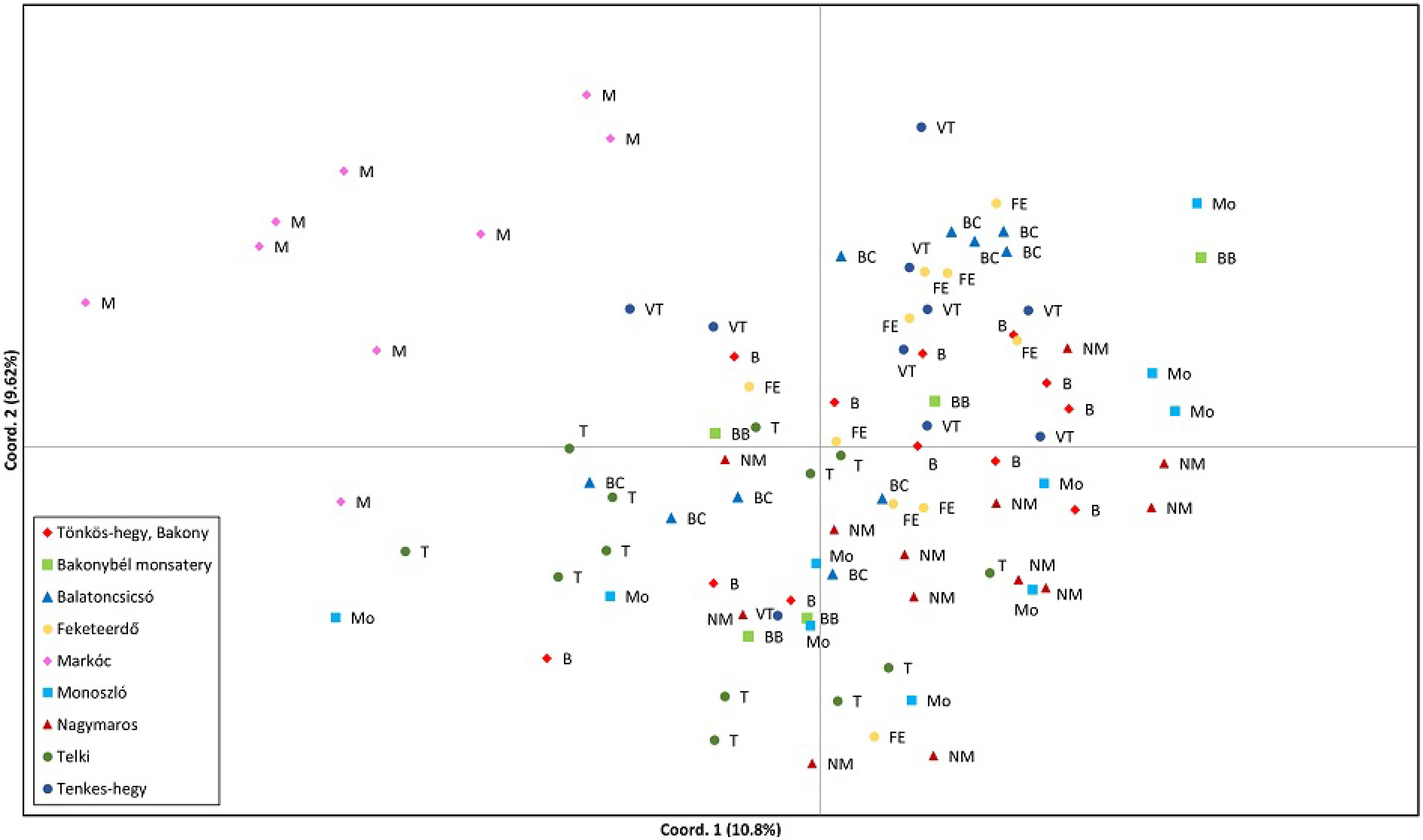
Figure 2.
Principal coordinate analysis (PCoA) of the cornelian cherry individuals collected from nine Hungarian populations. Individuals are colored by population. The first two axes explain 10.8% and 9.62% of the variance, respectively.
-
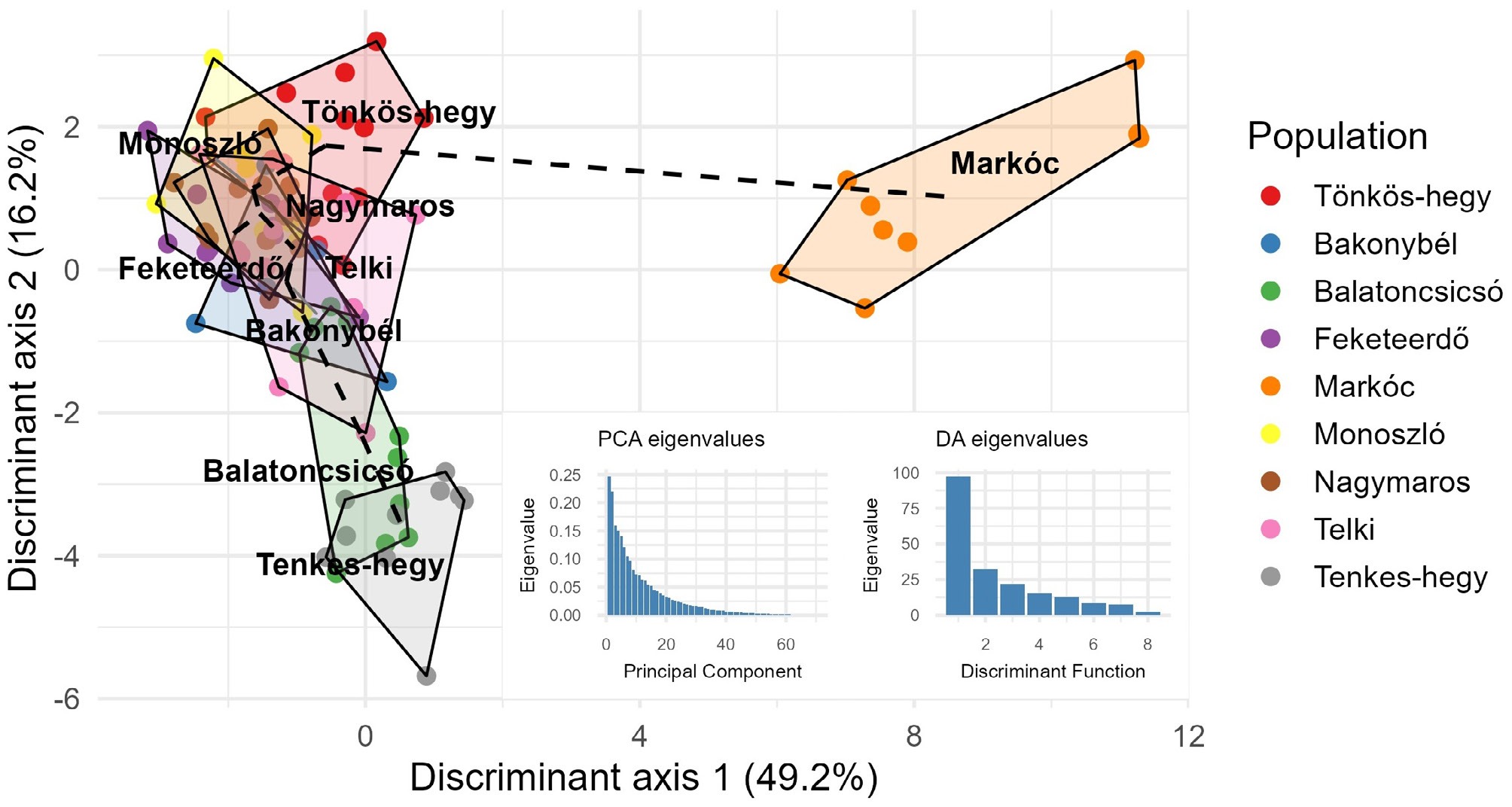
Figure 3.
Discriminant analysis of principal components (DAPC) with minimum spanning tree (MST). Individuals are colored by population, with polygons indicating clusters. The first two discriminant axes explain 49.2% and 16.2% of the variance, respectively. Dashed lines represent the MST connecting populations. Insets show eigenvalue distributions for PCA and discriminant functions.
-
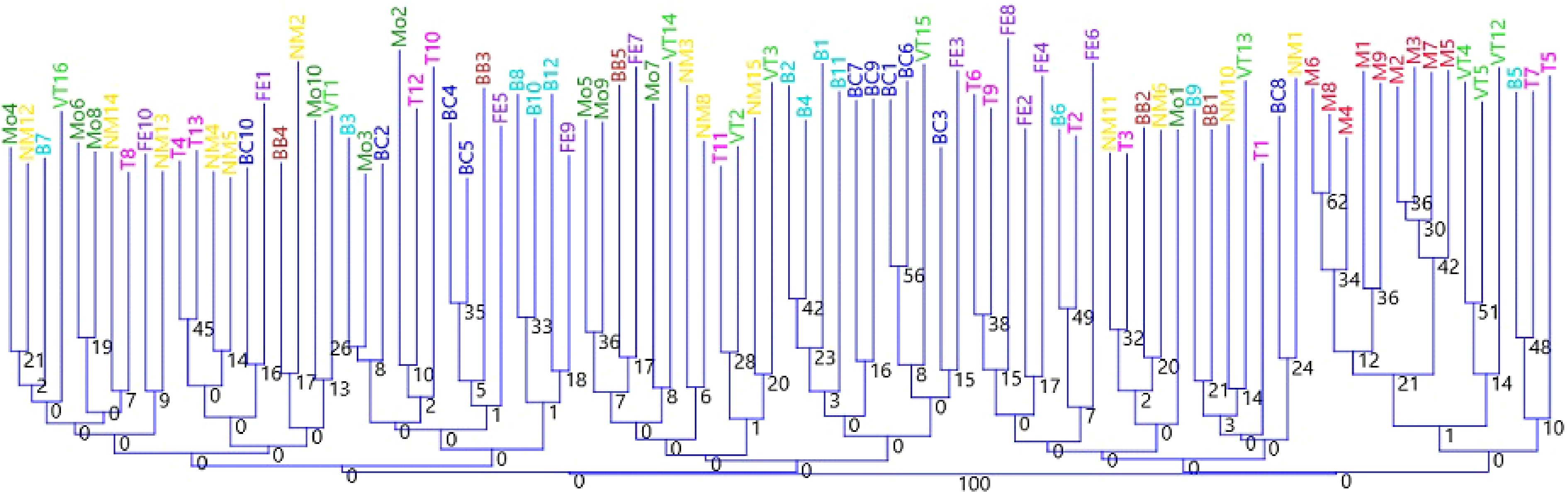
Figure 4.
Genetic distance of the studied Hungarian C. mas accessions using six SSR markers. Individuals are colored by population (B-Bakony, Tönkös-hegy = light blue, BB-Bakonybél monastery = brown, BC-Balatoncsicsó = dark blue, FE-Feketeerdő = purple, M-Markóc = red, MO-Monoszló = dark green, NM-Nagymaros = yellow, T-Telki = pink, VT-Tenkes-hegy = light green). The dendrogram was constructed by Neighbor joining method based on Jaccard similarity index. The numbers at specific nodes indicate percentage of 2000 bootstrap replicates in which a given group was found.
-
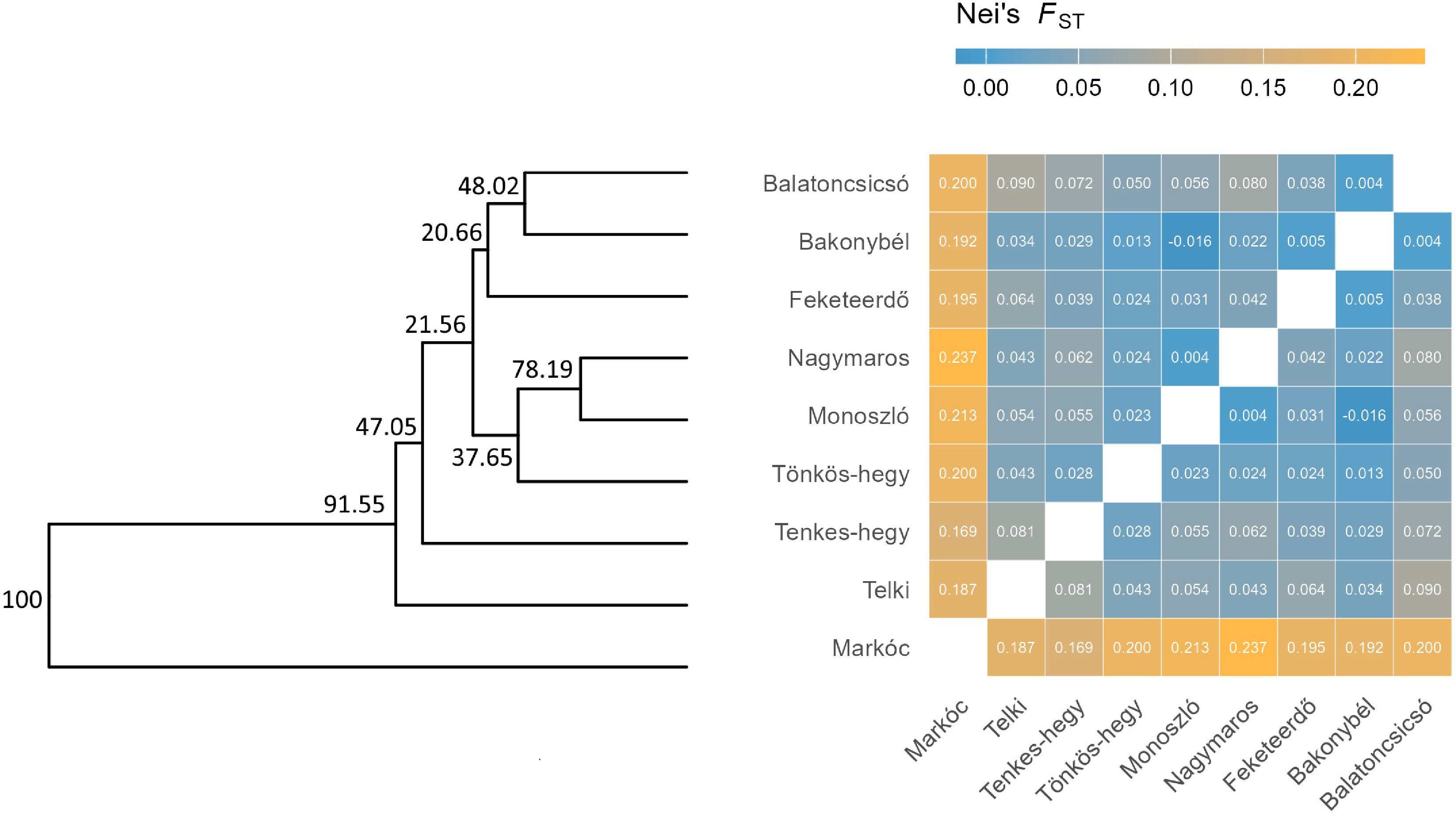
Figure 5.
UPGMA dendrogram and Nei's FST heatmap for Hungarian C. mas populations. The dendrogram (left) shows hierarchical clustering based on genetic distances, with bootstrap values indicating branch support. The heatmap (right) displays pairwise Nei's FST values, where color intensity reflects the degree of genetic differentiation (blue = low, orange = high). Higher FST values (> 0.18) indicate strong differentiation, while lower values (< 0.05) suggest closer genetic relationships among central populations.
-
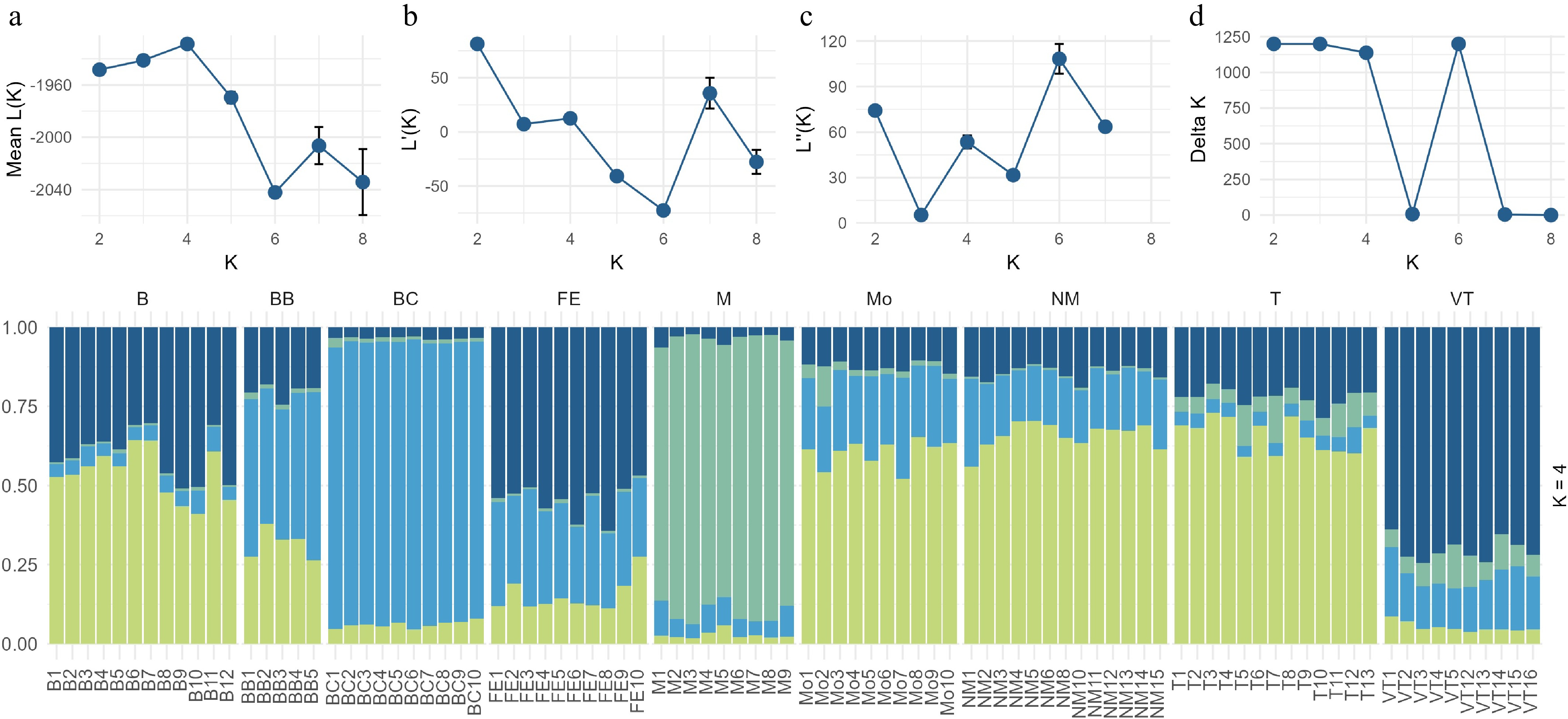
Figure 6.
Analysis of Hungarian cornelian cherry populations using STRUCTURE v2.3.4. Top: Model choice metrics for K = 2–8, including (a) mean log-likelihood, (b) its standard deviation, (c) second-order rate of change, and (d) ΔK, indicating K = 4 as optimal. Bottom: Barplot of individual assignment probabilities for K = 4. Each vertical bar represents an individual, and colors indicate membership proportions in each genetic cluster.
-
Code No. of
samplesLocation County GPS coordinates B 12 Tönkös-hegy Veszprém 47.267052, 17.731369 BB 5 Bakonybél Veszprém 47.251345, 17.727807 BC 10 Balatoncsicsó Veszprém 46.933607, 17.666828 FE 10 Feketeerdő Győr-Moson-Sopron 47.935377, 17.272106 M 9 Markóc Baranya 45.864789, 17.757312 MO 10 Monoszló Veszprém 46.906460, 17.641493 NM 13 Nagymaros Pest 47.795524, 18.944578 T 13 Telki Pest 47.538695, 18.856101 VT 10 Tenkes-hegy Baranya 45.891071, 18.248926 B = Bakony, Tönkös-hegy; BB = Bakonybél monastry; BC = Balatoncsicsó; FE = Feketeerdő; M = Markóc; MO = Monoszló; NM = Nagymaros; T = Telki; VT = Tenkes-hegy. Table 1.
The studied Hungarian cornelian cherry accessions with their geographical location.
-
Locus Primer sequence Repeat motif Ref. CF48 L: GCTTTGACATCCTCTTTGCTTCTC (TG)9 [15] R: AAGAGGCTTCACAAGACAATCAGC CF51 L: GGGCTAGTAGGTCGAGTGATCAAA (AG)7(GT)10 [15] R: CATTGCTTGGTGGTGATCTCTAAA CF55 L: TGGAGTAGGGCAAAAGATCAAGAG (GT)7T(TG)10 [15] R: TCCAGGGAATGTTCGGTAGATTAG CF59 L: TGGACTATAACGAGCAAGAAAGCA (AAAG)4 [15] R: GCTTTGTCCATAATCGTTTAGGCT CM007 L: GTTTAGGTGTGAGTGCAGATGG (GT)24 [18] R: CAATGCTAACAAGCACCATTCC CM008 L: TCGTTAATGTGAAATTGGAACG (GT)11 [18] R: CACCGTACACGCAAAGTCC CM010 L: GCTAGCAGAAGCACAGTTAGCC (CA)12 [18] R: TCCAACATGTAAAACCTAGATGC CM026 L: GAATTCATGTAATGTTGTTGTCTGC (CA)14 [18] R: CCTGCATATAATTCAGGTAAAGAGC CM031 L: TACCCTCTCTTGCTCTTTGTCC (AG)26(TG)13 [18] R: AAACAATCAAACCCAAACAACC CM037 L: AACACAGAGAAACACGTGCAA (TG)20 [18] R: TGGAGATCTTTGAAGAACAGGA CM039 L: GGGTATTGTAATCAATGTAAAACCAA (GT)18 [18] R: TCACACCACCAGCAATCACT CM043 L: GTCCACACCTGTTGTTCAGC (TG)16(TA)5 [18] R: GGTTGCAATGCTTTCTTGGT Table 2.
SSR loci used in this study, with forward and reverse primer sequences, repeat motifs, and references.
-
CF55 CM08 CM26 CM31 CM37 CM43 Average Expected size 155 156 192 208 184 220 − Obtained size 137–165 152–175 179–201 180–221 171–202 206–232 − Na 5 9 16 23 15 11 13.17 Ne 1.615 7.52 5.041 8.584 4.144 3.291 5.03 I 0.764 2.079 1.943 2.529 1.884 1.543 1.79 Ho 0.359 0.793 0.804 0.891 0.783 0.565 0.7 He 0.381 0.867 0.802 0.884 0.759 0.696 0.73 PIC 0.483 0.867 0.813 0.886 0.778 0.718 0.757 FIS 0.058 0.085 −0.003 −0.009 −0.032 0.188 0.048 Na = Number of different alleles, Ne = Number of effective alleles, I = Shannon's Information Index, Ho = Observed heterozygosity, He = Expected heterozygosity, PIC = Polymorphic Information Content, FIS = Wright's inbreeding coefficient. Table 3.
Expected and observed allele size ranges and genetic diversity parameters of the six studied SSR loci.
Figures
(6)
Tables
(3)