-
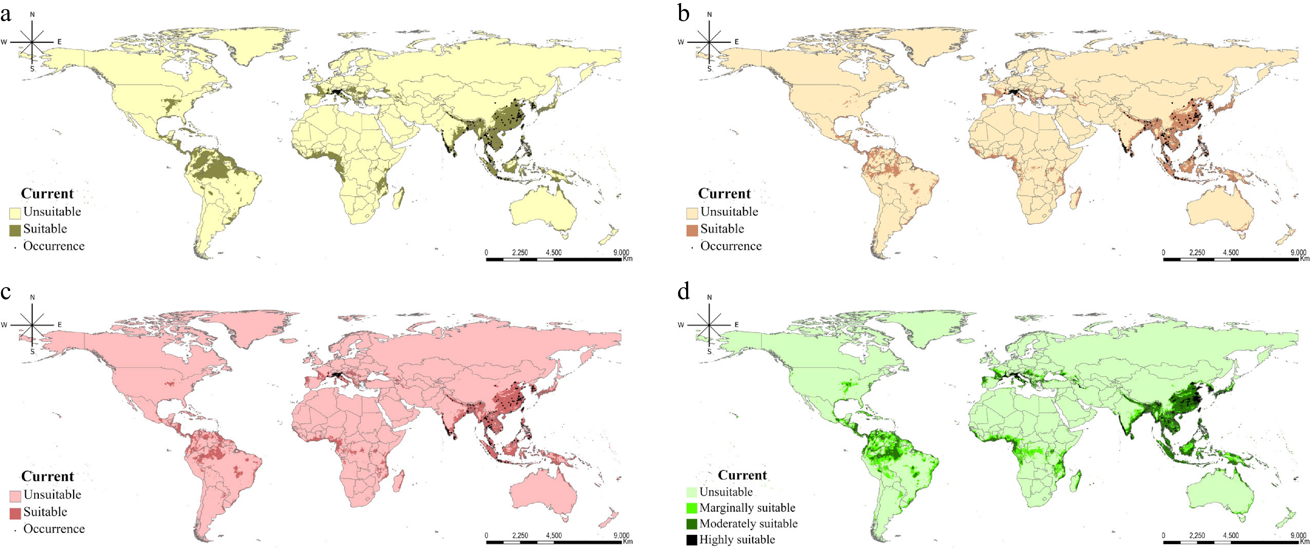
Figure 1.
Current distribution of R. speculum as predicted by three machine learning algorithms and their TSS-weighted ensemble: (a) MaxEnt, (b) Random Forest, (c) XGBoost, and (d) the TSS-weighted ensemble suitability map integrating the three algorithms. The source of the map layout was obtained from ArcGIS Pro 3.6.0 software (
www.arcgis.com/home/index.html ). -
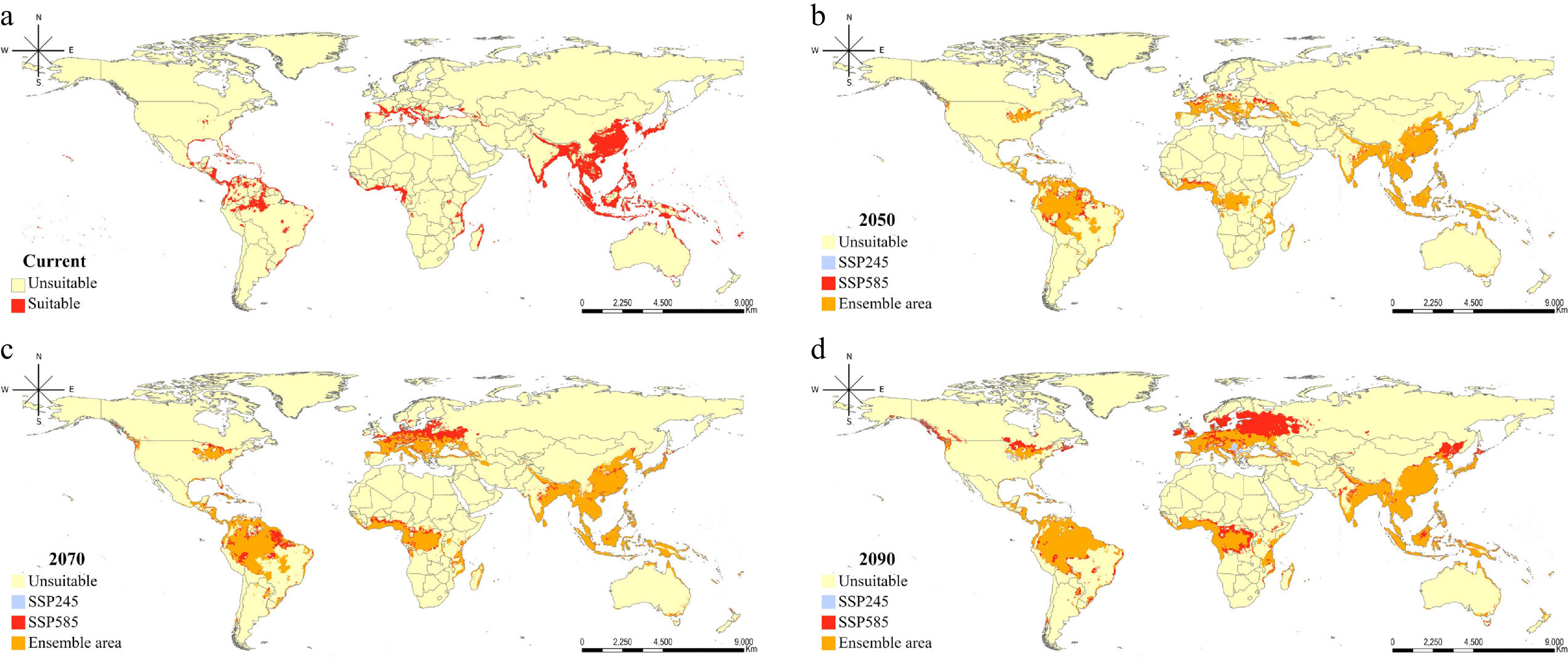
Figure 2.
Ensemble projection of three different machine learning algorithms for the potential distribution of R. speculum according to climate change scenarios: (a) Current, (b) 2041–2060, (c) 2061–2080, and (d) 2081–2100. Ensemble areas are those projected to have moderate suitability by the ensemble methods. The source of the map layout was obtained from ArcGIS Pro 3.6.0 software (
www.arcgis.com/home/index.html ). -
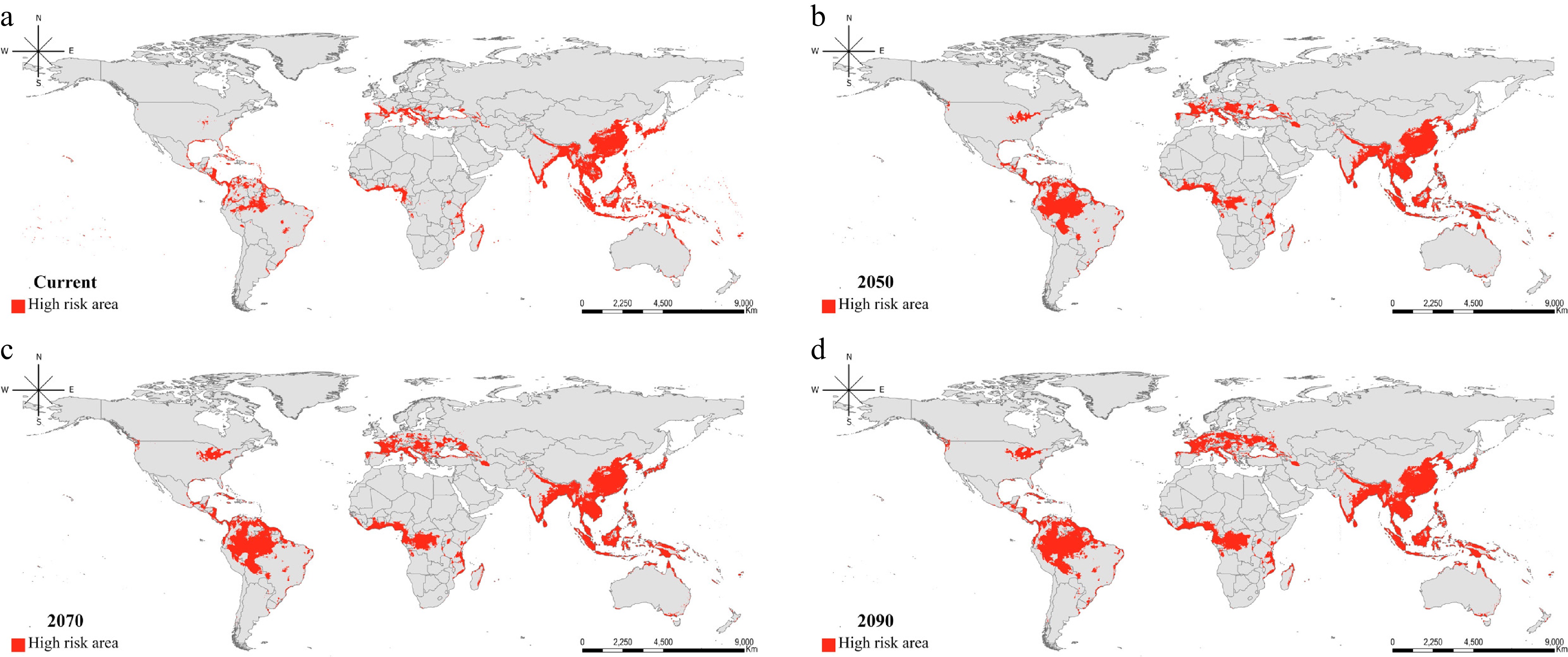
Figure 3.
Projected sustainable risk regions identified to have moderate suitability by the ensemble approach across climate change scenarios and different modeling algorithms: (a) Current, (b) 2041–2060, (c) 2061–2080, and (d) 2081–2100. The source of the map layout was obtained from ArcGIS Pro 3.6.0 software (
www.arcgis.com/home/index.html ). -
Variables Description Percent contribution (%) MaxEnt (%)* Random Forest** XGBoost*** Bio1 Annual mean temperature 19.1 35.4 0.032 0.18 Bio2 Mean diurnal range 26.2 28.4 0.018 0.174 Bio5 Max temperature of warmest month 0.4 4.9 0.021 0.058 Bio8 Mean temperature of wettest quarter 2.1 2.4 0.02 0.041 Bio12 Annual precipitation 23.9 23.8 0.025 0.315 Bio14 Precipitation of driest month 0.5 1.2 0.016 0.054 Bio15 Precipitation seasonality 0.5 2.2 0.012 0.058 Bio18 Precipitation of warmest quarter 1.2 1.4 0.023 0.068 Bio19 Precipitation of coldest quarter 0.1 0.3 0.012 0.052 * In MaxEnt, variable contribution represents the accumulated increase in regularized gain attributable to each variable across all iterations of the algorithm.
** In RF, it is measured by permutation importance, which represents the decrease in predictive accuracy on out-of-bag samples when the values of a variable are randomly permuted.
*** In XGBoost, it is quantified by average gain, which measures the mean reduction in the objective function loss contributed by each variable when used as a splitting node across all trees.Table 1.
Selected bioclimatic variables and their contributions for R. speculum.
-
Model Hyperparameter Description Grid search ranges Selected values Random Forest Number of trees Number of trees in the forest 300, 500, 700, 1,000 1,000 Mtry Number of variables sampled at each split 2, 3, 4, 5 3 Node size Minimum node size 1, 3, 5, 7 1 XGBoost Eta (η) Learning rate 0.05, 0.1 0.05 Max depth Maximum depth 3, 5, 7 7 Gamma (γ) Minimum loss reduction 0, 0.25, 0.5 0.25 Colsample by tree Feature subsampling 0.6, 0.8, 1.0 1 Min child weight Minimum sum of instance weight 1, 3, 5 3 Subsample Data subsampling 0.6, 0.8, 1.0 0.6 n estimators Number of trees 1~2,000 332* * The optimal number of trees was determined as 332 using early stopping (tolerance = 50). Table 2.
Hyperparameter settings and optimal values for RF and XGBoost.
-
Sensitivity Specificity Accuracy AUC TSS MaxEnt 0.967 0.886 0.886 0.951 0.853 Random Forest 0.972 0.898 0.901 0.978 0.87 XGBoost 0.968 0.905 0.908 0.979 0.874 Table 3.
Performance metrics of the three SDM algorithms for R. speculum under current climate conditions.
-
Current (%) 2050 2070 2090 Sustained area** SSP245 SSP585 SSP245 SSP585 SSP245 SSP585 MaxEnt 64,180 (11.09) 68,427 (11.82) 74,709 (12.91) 76,139 (13.15) 92,468 (15.97) 81,070 (14) 114,497 (19.78) 47,467 (8.2) Random Forest 53,603 (9.26) 72,182 (12.47) 84,955 (14.68) 84,761 (14.64) 112,042 (19.35) 93,418 (16.14) 151,000 (26.08) 38,771 (6.7) XGBoost 51,242 (8.85) 66,116 (11.42) 74,708 (12.91) 74,521 (12.87) 93,302 (16.12) 80,215 (13.86) 111,875 (19.33) 36,269 (6.27) Ensemble** 43,921 (7.59) 56,532 (9.77) 64,839 (11.2) 64,959 (11.22) 83,680 (14.46) 71,084 (12.28) 104,000 (17.97) 31,831 (5.5) * Sustained area is defined as areas where the potential for occurrence persists under climate change, calculated on the basis of the total number of pixels = 578,888. ** Regions with moderate suitability. Table 4.
Temporal projections of suitable habitat extent for R. speculum, represented by pixel counts across multiple models and climate trajectories.
Figures
(3)
Tables
(4)