-
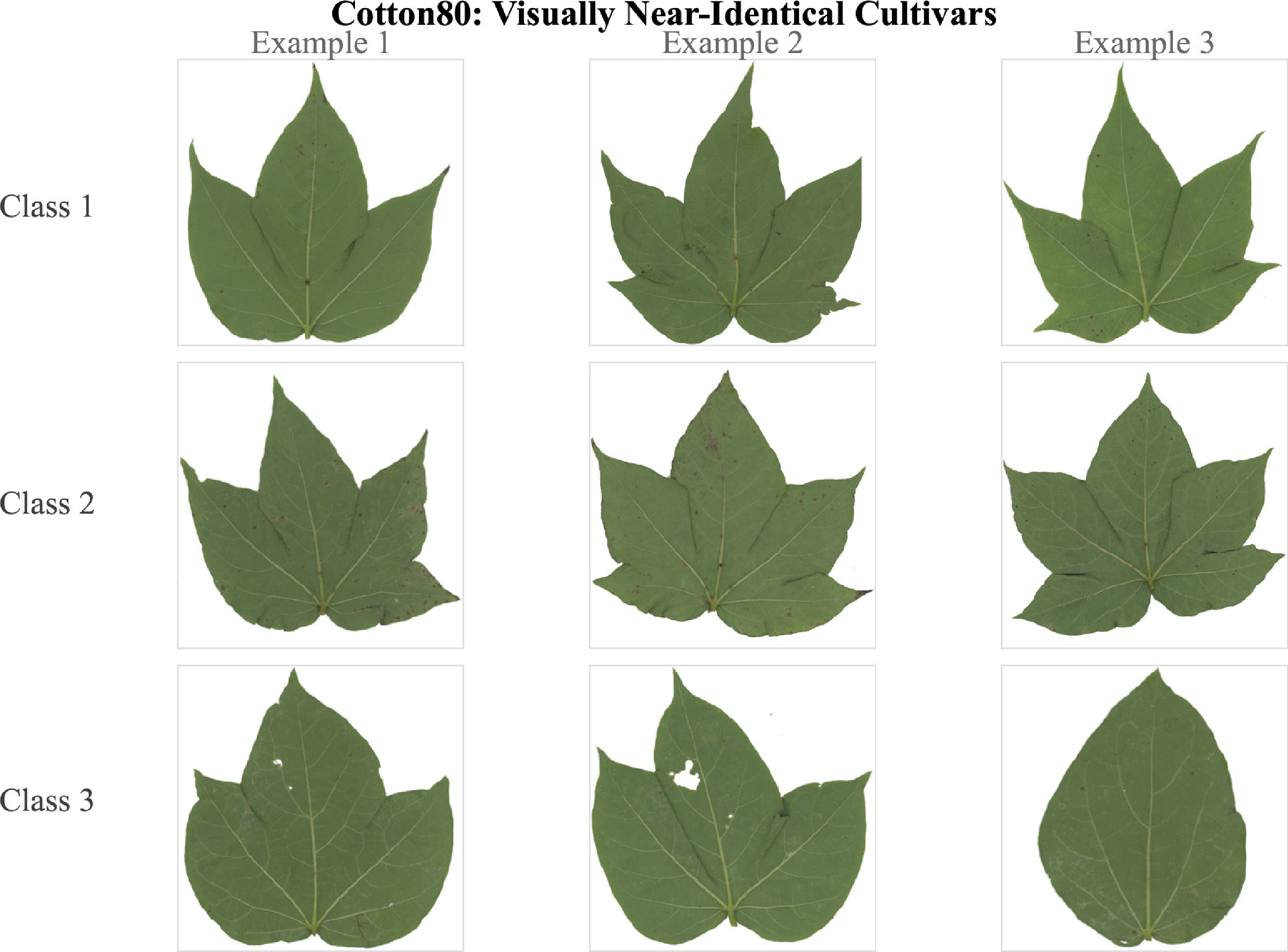
Figure 1.
Representative images from the Cotton80 cultivar classes (three images per class)[1]. Despite belonging to distinct cultivar categories, samples share near-identical macro-morphology: a defining characteristic of Ultra-FGVC that limits even state-of-the-art supervised methods to below 60% accuracy at K = 50. The figure is original and created by Chenhui Wang. © 2026 Chenhui Wang.
-
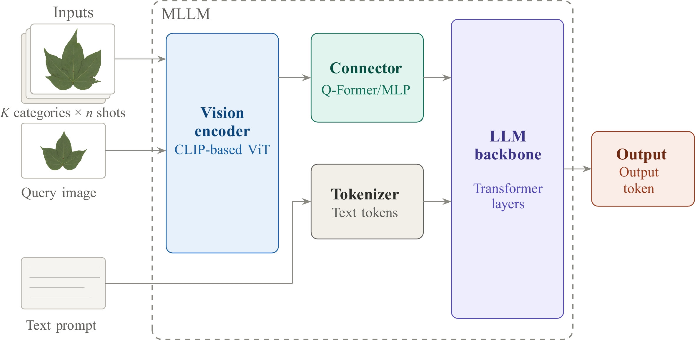
Figure 2.
Base architecture of a multimodal large language model (MLLM) for few-shot in-context learning. Reference images [1] (K categories, n shots each) and an unlabelled query image are encoded by a CLIP-based vision encoder[33], whose patch features are projected into the language model's token space by a lightweight cross-modal connector (Q-Former[35] or MLP bridge[11]). A text prompt encoding the task instruction and category identifiers is tokenised in parallel. Both token streams are consumed jointly by the LLM backbone, which generates a structured output containing the predicted category label. In this work, category identifiers are numeric only (Task 1) or real species names (Task 2); the backbone architecture is otherwise identical across conditions. The figure is original and created by Chenhui Wang. © 2026 Chenhui Wang.
-
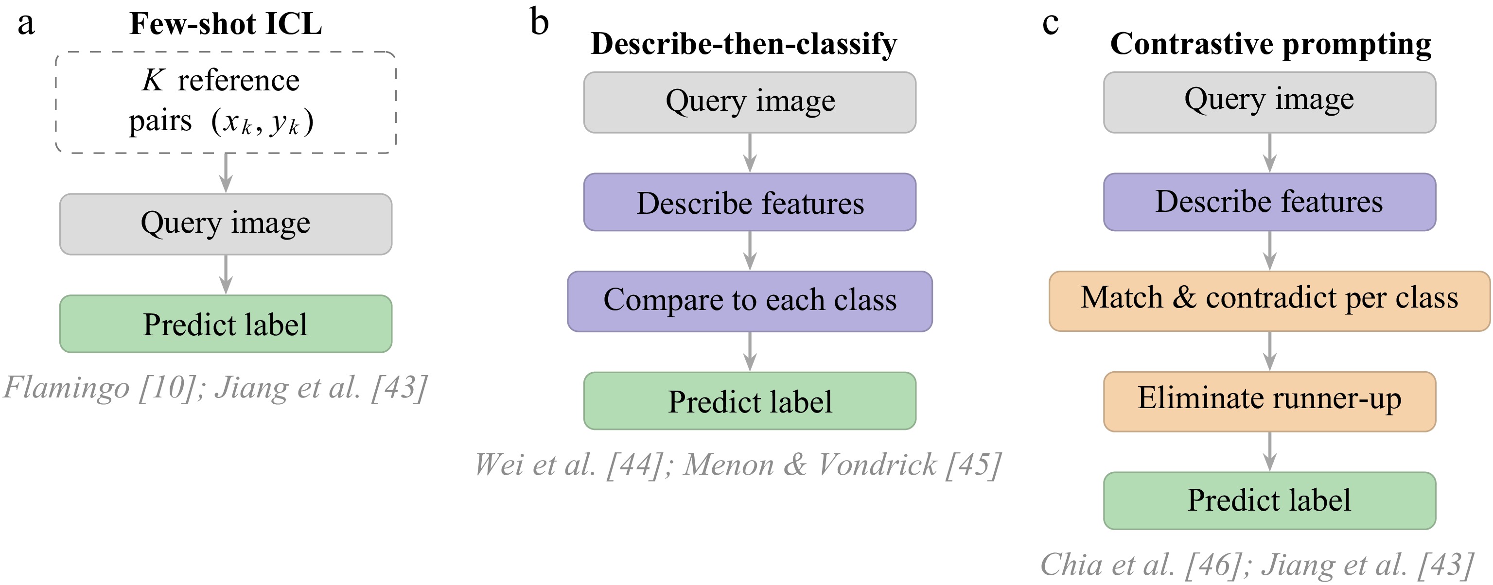
Figure 3.
Structural comparison of the three prompting paradigms reviewed in this section. (a) Few-shot ICL prepends
$ K $ $ ({\bf{x}}_k, y_k) $ -
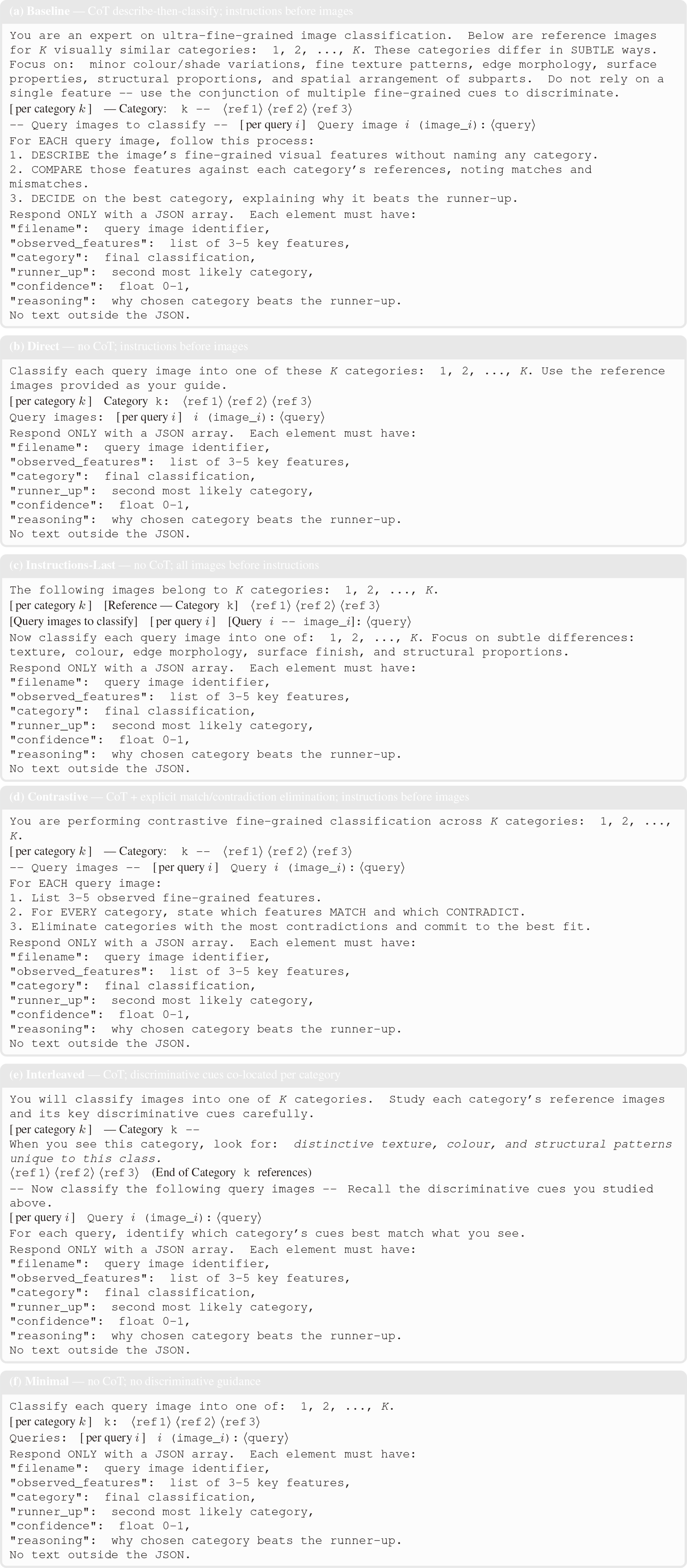
Figure 4.
All six prompt variants used in Task 3, shown schematically (part 1 of 2: variants a–c). Image blocks are denoted
$ \langle\,\cdot\,\rangle $ -
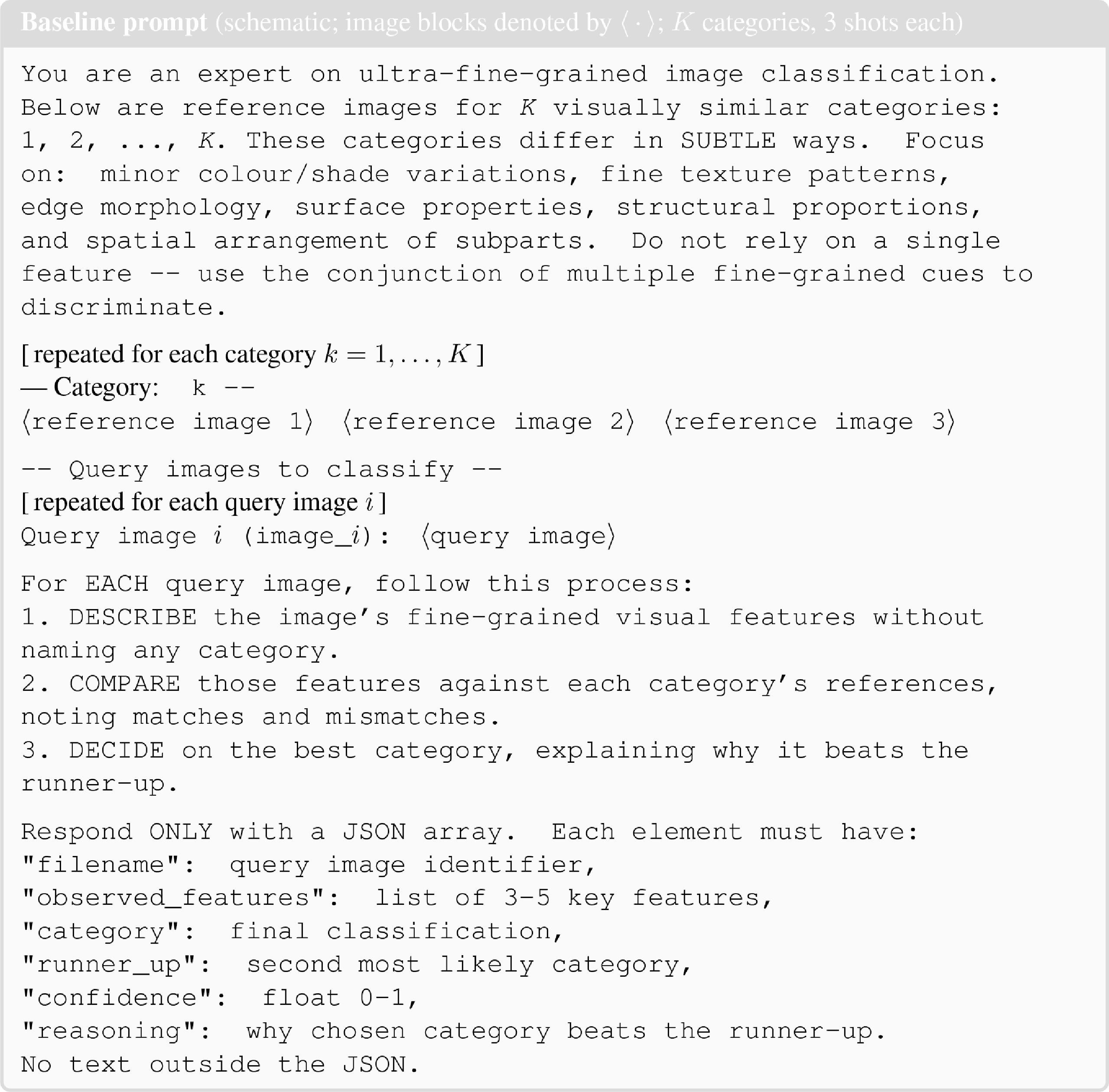
Figure 5.
Full baseline prompt used in Tasks 1–3. Italicised
$ K $ -
Table 1.
MLLMs evaluated in this study. Version strings are exact API identifiers used in all experiments.
-
Variant CoT Contrastive Instruction placement Role Baseline $ \checkmark$ – Preamble (before images) Primary reference; describe-then-classify[45] Contrastive $ \checkmark$ $ \checkmark$ Preamble (before images) Adds per-category match/contradiction elimination[46,47] Interleaved $ \checkmark$ – Co-located per category Tests local vs global instruction placement Instructions-Last – – Appended (after all images) Tests effect of deferred instructions on attention Direct – – Preamble (before images) Isolates CoT contribution; no reasoning steps Minimal – – Inline with images Lower bound; no discriminative guidance CoT = chain-of-thought describe-then-classify decomposition; Contrastive = per-category match/contradiction elimination; Instruction placement = where task instructions appear relative to the images. Table 2.
Summary of the six prompt variants.
-
Method $ K = 3 $ $ K = 10 $ $ K = 50 $ SoyLocal Supervised methods (fine-tuned) Human Expert 63.89 32.50 12.84 AlexNet[29] 88.89 53.33 33.33 VGG-16[59] 77.78 50.00 56.00 ResNet-50[28] 88.89 63.33 62.00 DCL[60] 88.89 63.33 60.67 MLLMs, few-shot ICL (this work) gemini-3-flash-preview[22] 85.56 ± 12.01 46.00 ± 6.81 — gpt-5.4-2026-03-05[21] 81.67 ± 15.41 51.67 ± 9.72 20.44 ± 3.79 $ ^{\,\ddagger} $ kimi-k2.5[20] 82.78 ± 13.23 45.00 ± 7.24 — qwen3.5-397b-a17b[23] 79.45 ± 19.17 46.67 ± 10.30 — Cotton80 Supervised methods (fine-tuned) Human Expert 66.67 63.33 14.00 AlexNet[29] 88.89 66.67 24.67 VGG-16[59] 77.78 56.67 53.33 ResNet-50[28] 88.89 66.67 52.67 DCL[60] 77.78 73.33 54.67 MLLMs, few-shot ICL (this work) gemini-3-flash-preview[22] 67.78 ± 13.44 33.67 ± 12.42 — gpt-5.4-2026-03-05[21] 71.67 ± 14.63 39.33 ± 8.13 12.44 ± 5.09 $ ^{ \ddagger} $ kimi-k2.5[20] 67.22 ± 16.31 34.00 ± 12.05 — qwen3.5-397b-a17b[23] 47.22 ± 26.46 34.33 ± 9.03 — Supervised baselines from Yu et al.[1]; MLLM results are mean ± standard deviation over N independent rounds under the blind numeric-label protocol. '—' indicates conditions not evaluated. At K = 3, the random-guessing baseline is 33.3%. $ \ddagger $ Table 3.
Top-1 accuracy (%) on SoyLocal and Cotton80.
-
Dataset Model $ K $ $ N $ $ \bar{A}_{B} $ $ \bar{A}_{N} $ $ \bar{\Delta} $ $ p $ $ d $ CUB-Crows gemini-3-flash-preview[22] 3 20 0.922 0.922 +0.000 1.000 0.00 gemini-3-flash-preview[22] 9 10 0.807 0.822 +0.015 0.533 0.20 gpt-5.4-2026-03-05[21] 3 20 0.883 0.889 +0.006 0.825 0.05 gpt-5.4-2026-03-05[21] 9 10 0.678 0.730 +0.052 0.050 0.72 qwen3.5-397b-a17b[23] 3 20 0.867 0.878 +0.011 0.629 0.11 qwen3.5-397b-a17b[23] 9 10 0.743 0.754 +0.004 0.883 0.05 kimi-k2.5[20] 3 20 0.845 0.883 +0.039 0.232 0.28 kimi-k2.5[20] 9 10 0.789 0.793 +0.004 0.868 0.05 CUB-Cormorant (K = 3 exhausts available categories; no ceiling effects) gemini-3-flash-preview[22] 3 20 0.678 0.778 +0.100 0.114 0.37 gpt-5.4-2026-03-05[21] 3 20 0.689 0.722 +0.033 0.516 0.15 qwen3.5-397b-a17b[23] 3 20 0.739 0.689 −0.050 0.359 −0.21 kimi-k2.5[20] 3 20 0.683 0.683 +0.000 1.000 0.00 $ \bar{A}_{B} $ $ \bar{A}_{N} $ $ \bar{\Delta} $ $ d $ $ d $ $ = \bar{\Delta}/s_\Delta $ $ p $ $ t $ $ \delta_r = A_{\mathrm{N}}^{(r)} - A_{\mathrm{B}}^{(r)} $ $ \alpha/m \approx 0.00417 $ $ m = 12 $ $ K = 9 $ $ n = 10 $ $ \approx 35\% $ $ d = 0.50 $ $ K = 3 $ $ n = 20 $ $ \bar{A} \geq 0.84 $ $ K = 3 $ $ n = 20 $ $ \bar{A}_{B} \leq 0.74 $ Table 4.
Task 2 paired-comparison statistics (blind vs named label condition).
-
Variant CoT Contr. Instr. Gemini-3-flash-preview Kimi-K2.5 Top-1 (%) Top-2 (%) Top-1 (%) Top-2 (%) Baseline $ \checkmark$ – Pre 41.3 ± 6.9 58.3 42.3 ± 8.9 64.7 Instructions-Last – – Post 38.3 ± 10.5 56.0 46.3 ± 7.1 68.7 Contrastive $ \checkmark$ $ \checkmark$ Pre 37.3 ± 15.9 61.5 48.0 ± 6.9 66.7 Minimal – – Inline 37.0 ± 20.0 65.0 39.0 ± 21.6 69.2 Interleaved $ \checkmark$ – Local 35.7 ± 13.7 61.1 48.7 ± 9.5 71.7 Direct – – Pre 35.0 ± 19.7 64.6 45.7 ± 17.1 68.9 Mean (all variants) 37.4 45.0 Top-1 and Top-2 accuracy: mean ± standard deviation. All rounds produced parseable output. The elevated standard deviations on Direct and Minimal (17%–22%) reflect genuine round-to-round variability under stochastic category sampling, not output failures. Instr. placement abbreviations: Pre = preamble before images; Post = appended after all images; Local = co-located per category; Inline = inline with images. Variants are ordered by Gemini top-1 accuracy (descending). Table 5.
Prompt ablation results on SoyLocal (n = 10 rounds per variant per model).
Figures
(5)
Tables
(5)