-
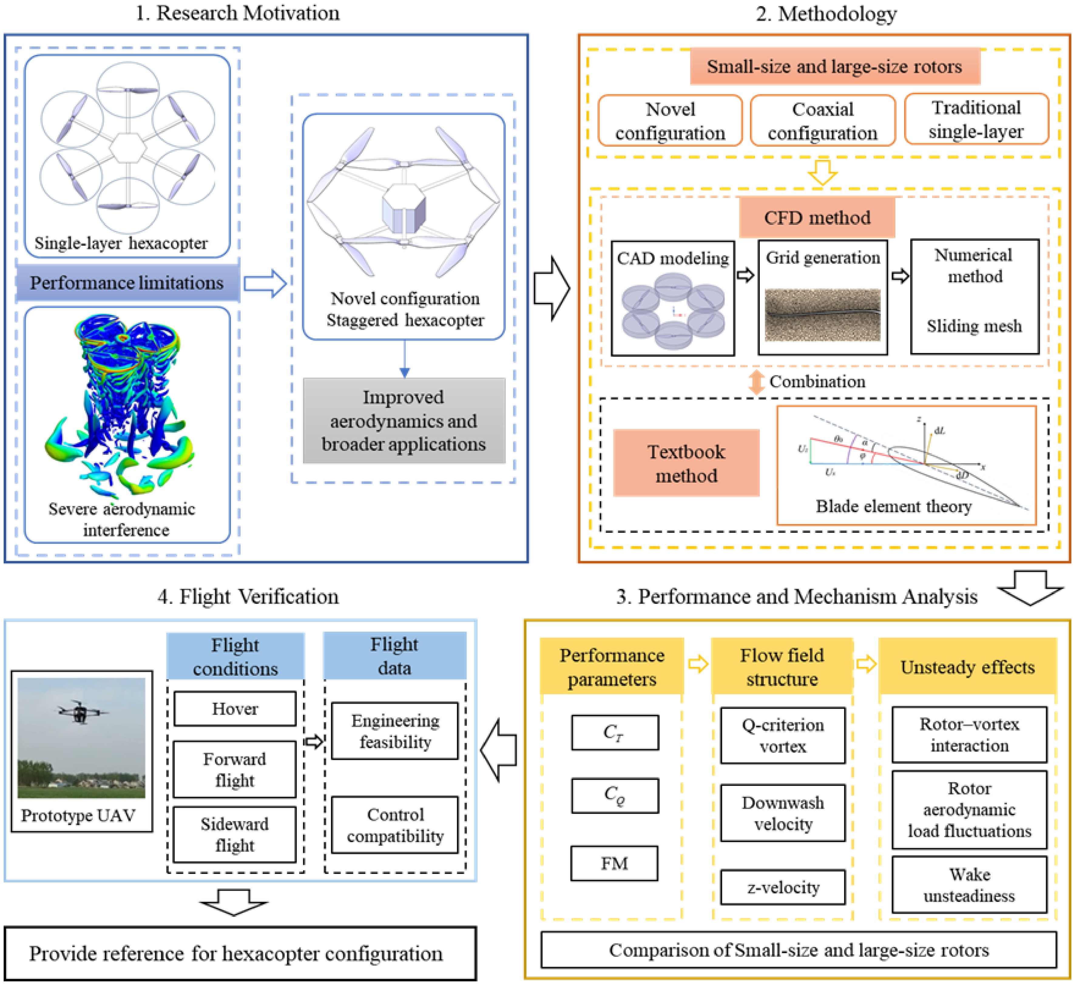
Figure 1.
Research logical relationship diagram.
-
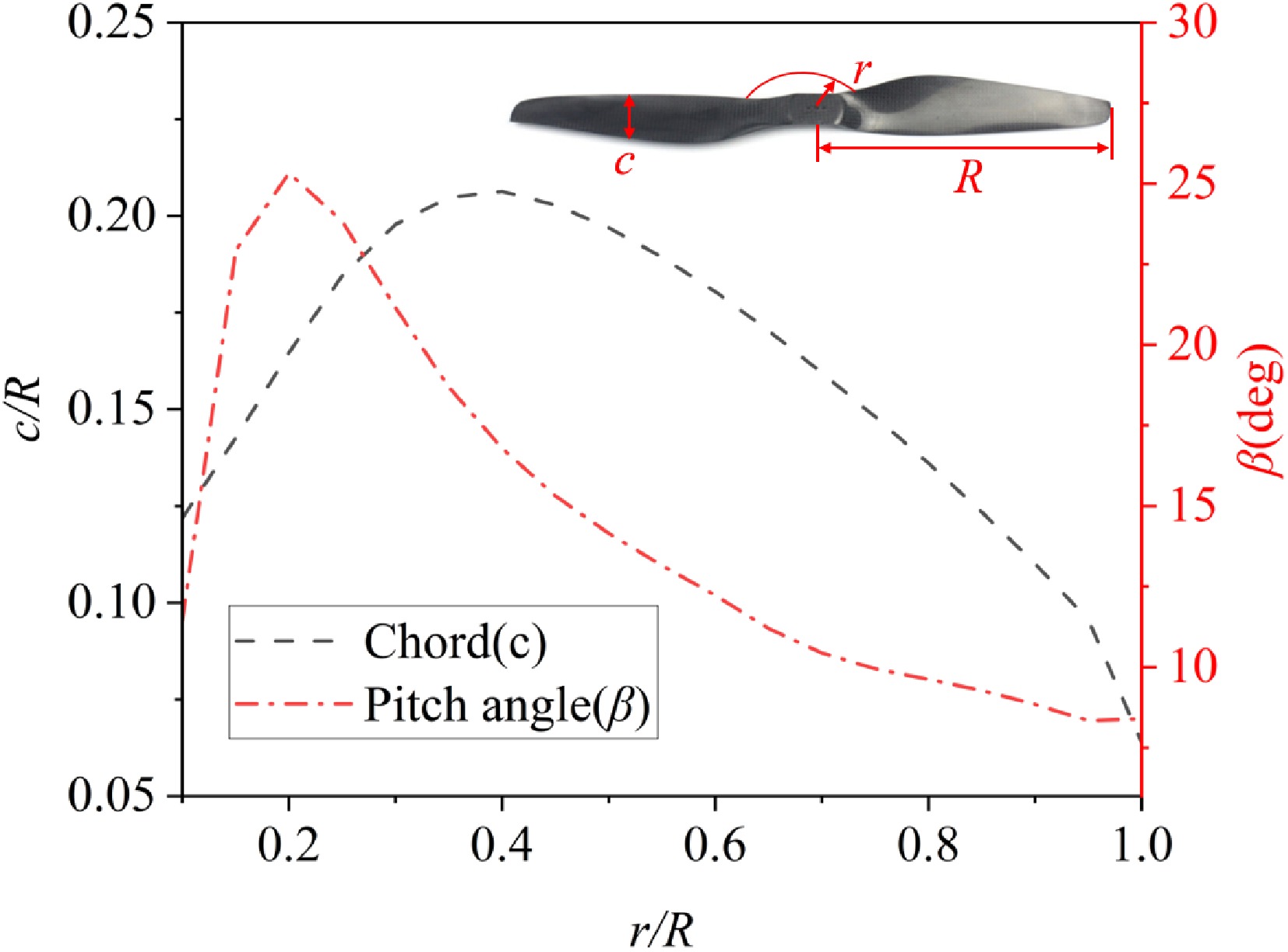
Figure 2.
Plot of propeller's chord (c) and pitch angle (β) distribution of the T-MOTOR 1855 propeller.
-
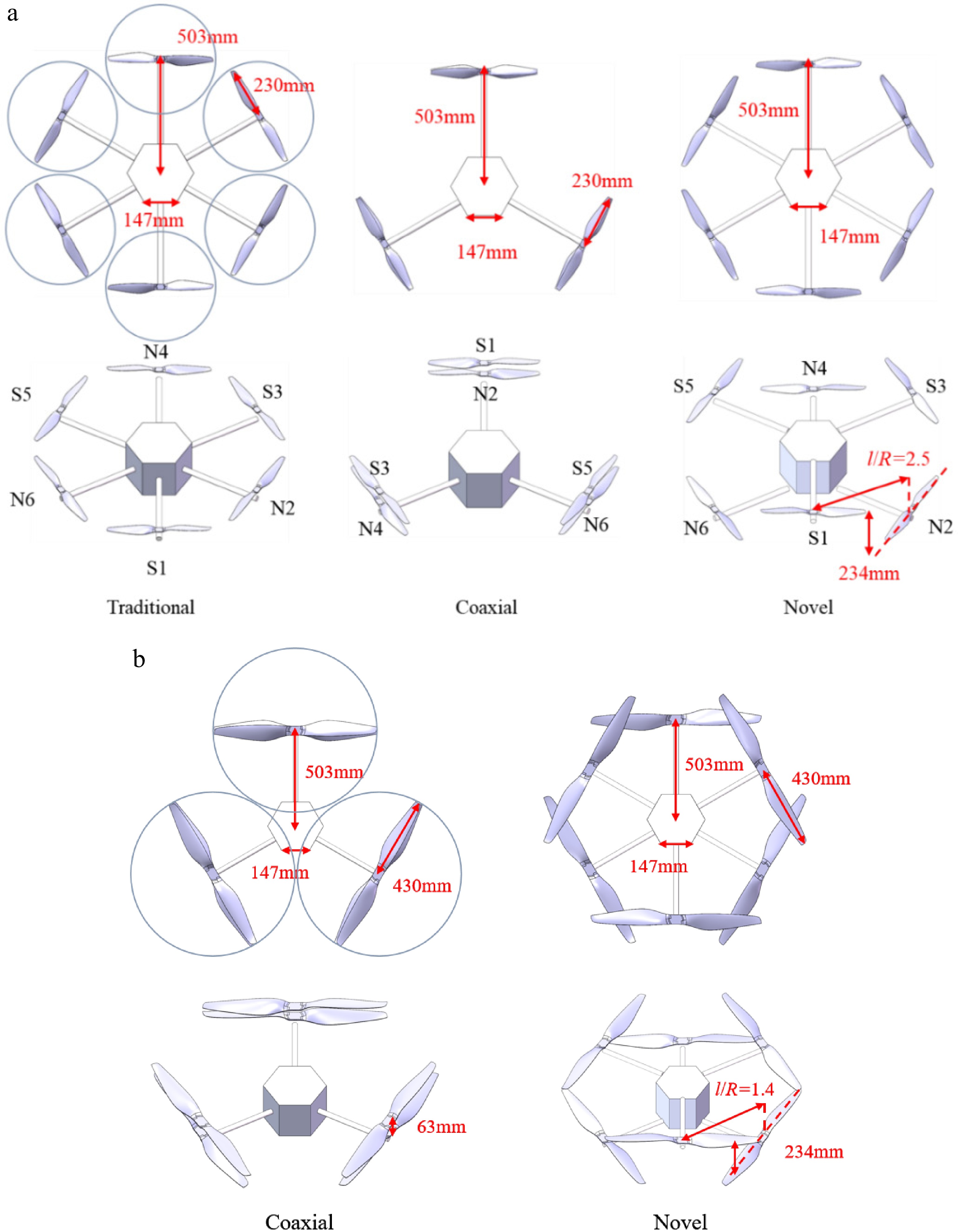
Figure 3.
Different hexacopter configurations. (a) Small-sized rotor. (b) Large-sized rotor.
-
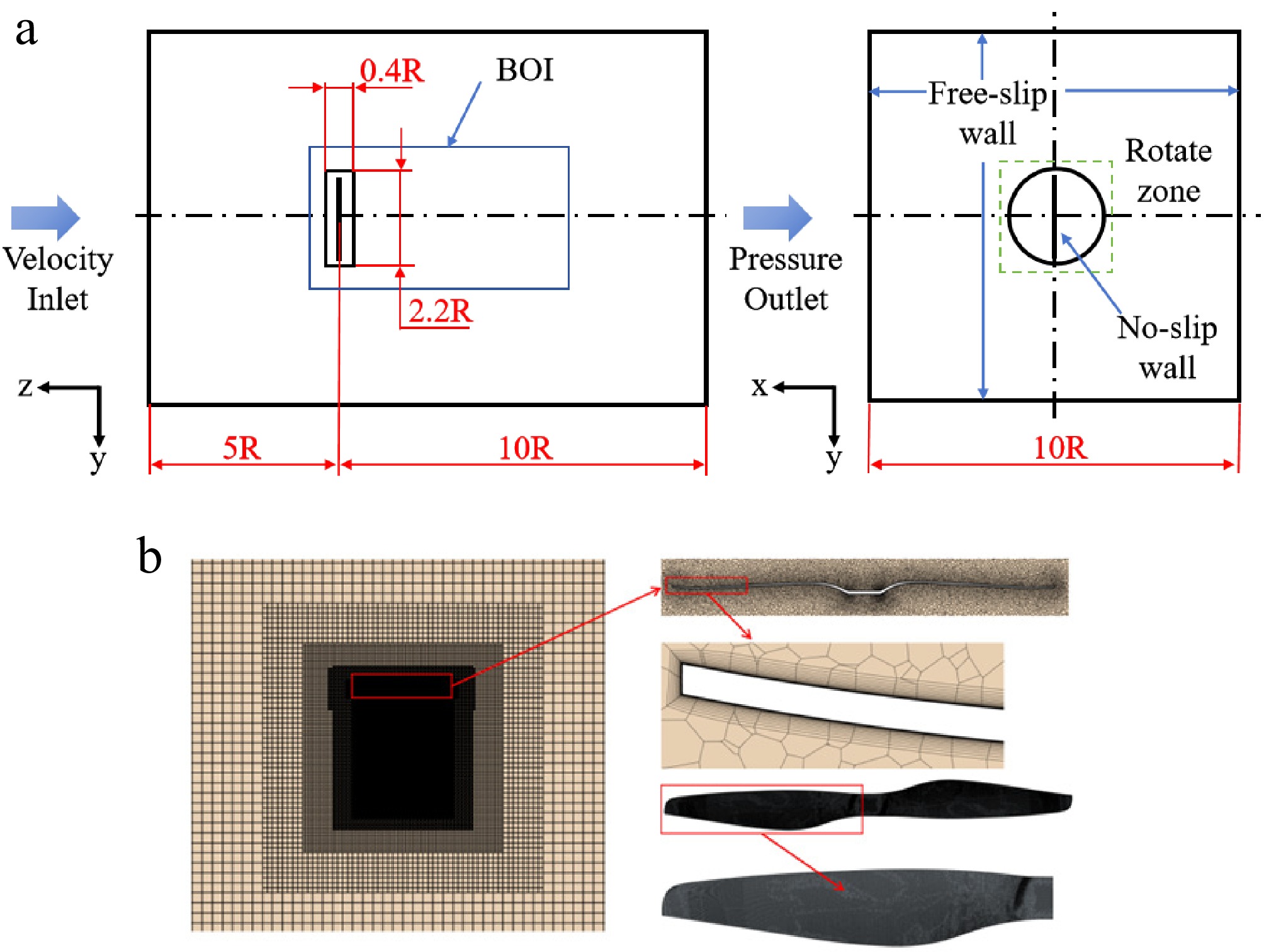
Figure 4.
Computational domain and mesh partitioning. (a) Computational domain and boundary conditions; (b) Computational mesh.
-
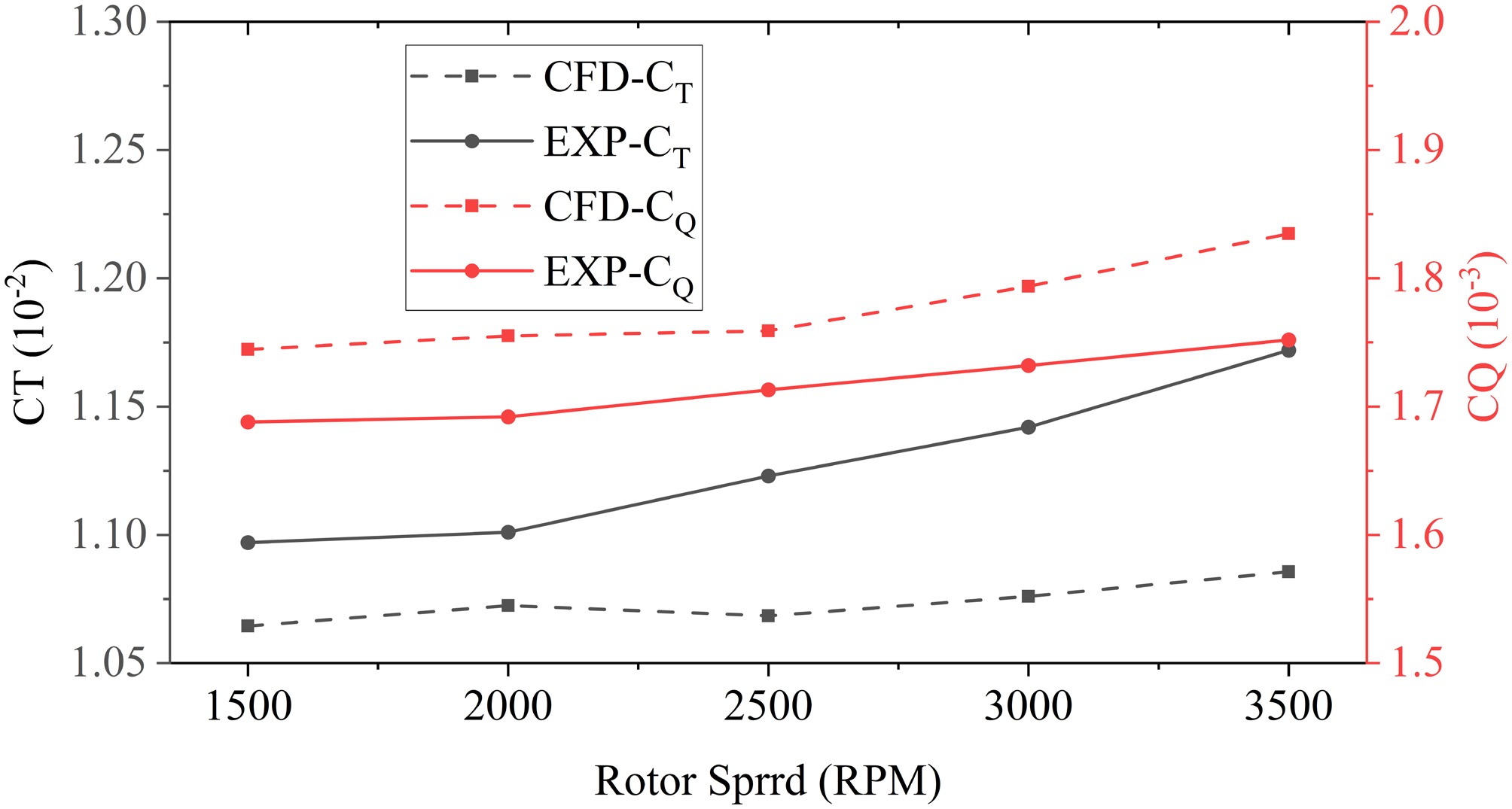
Figure 5.
Validation of thrust and torque coefficients for a single rotor.
-
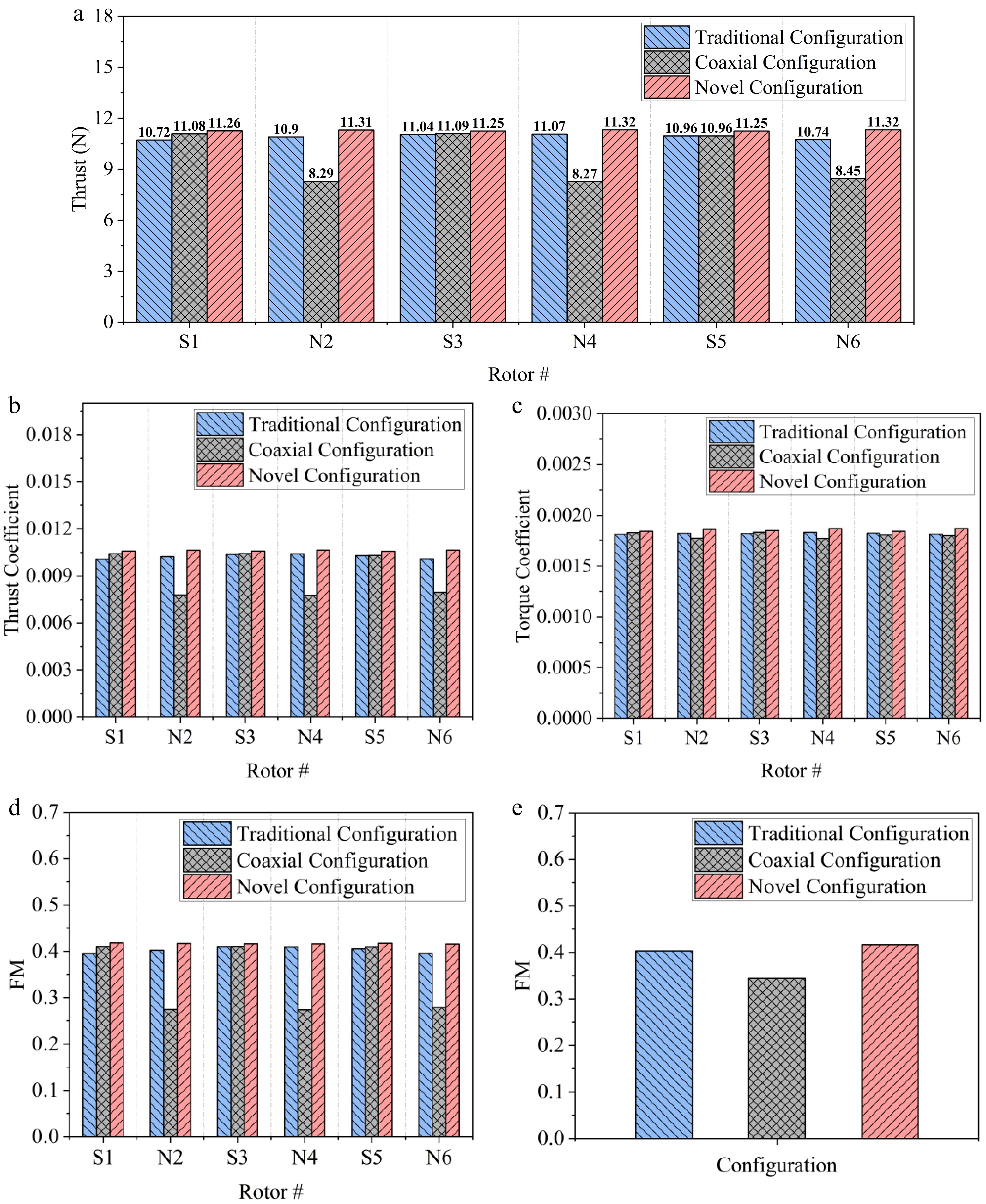
Figure 6.
Aerodynamic performance of three small-sized rotors. (a) Rotor thrust for various configurations. (b)Thrust coefficient. (c) Torque coefficient. (d) FM of each rotor. (e) Average FM of the hexacopter.
-
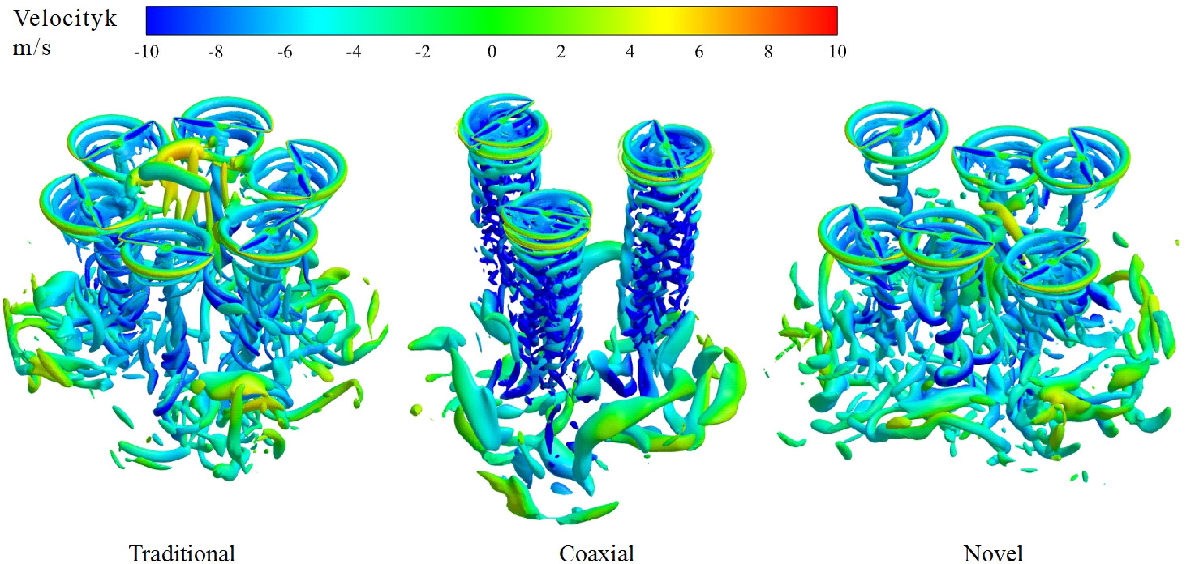
Figure 7.
Isosurface of Q-criterion and z-velocity for small-size rotors.
-
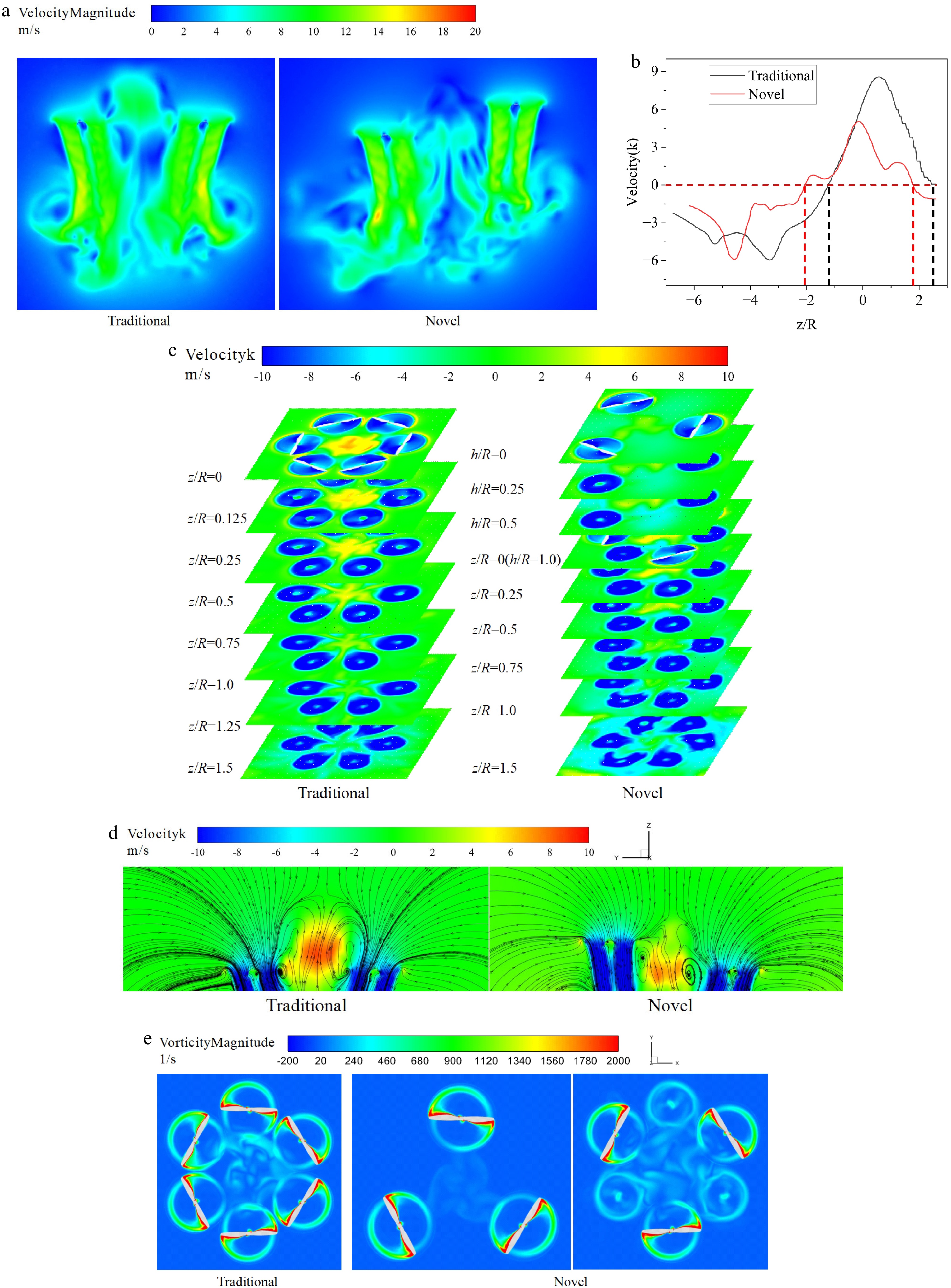
Figure 8.
(a) Downwash velocity distributions. (b) Axial velocity distribution along the z-axis in the central region of the hexacopter system. (c) z-Velocity distributions. (d) z-Velocity-streamline distributions. (e) Vorticity distribution at the rotor disk plane.
-
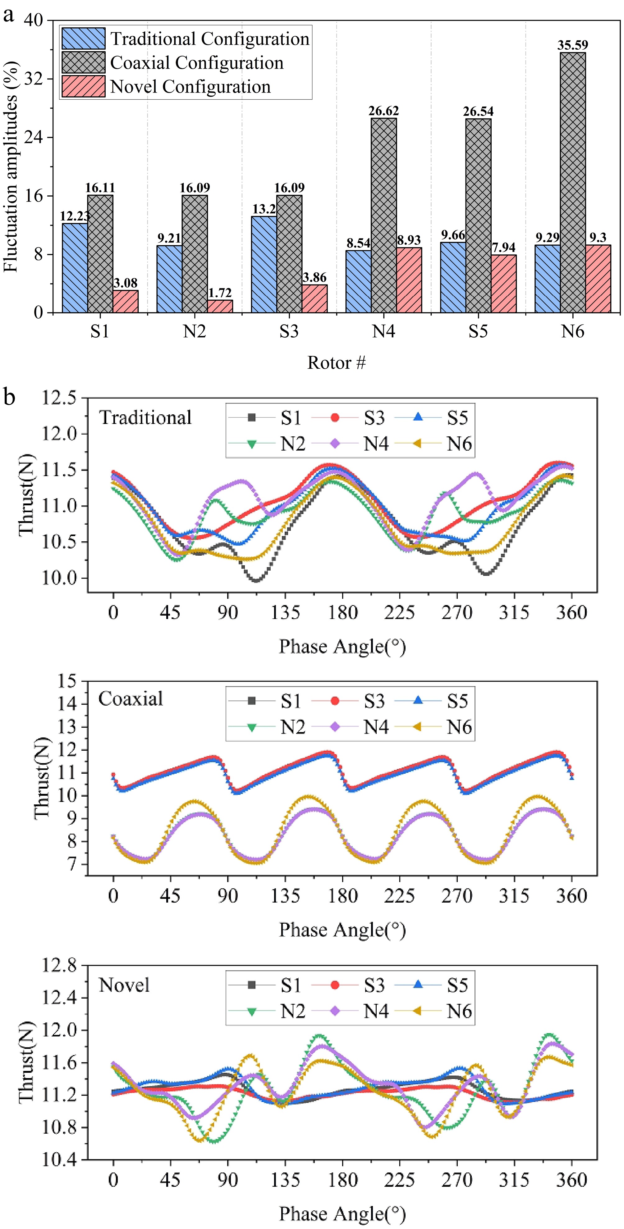
Figure 9.
(a) Ratios of peak-to-trough fluctuation amplitudes of instantaneous thrust to mean thrust. (b) Thrust variation with phase during one revolution.
-
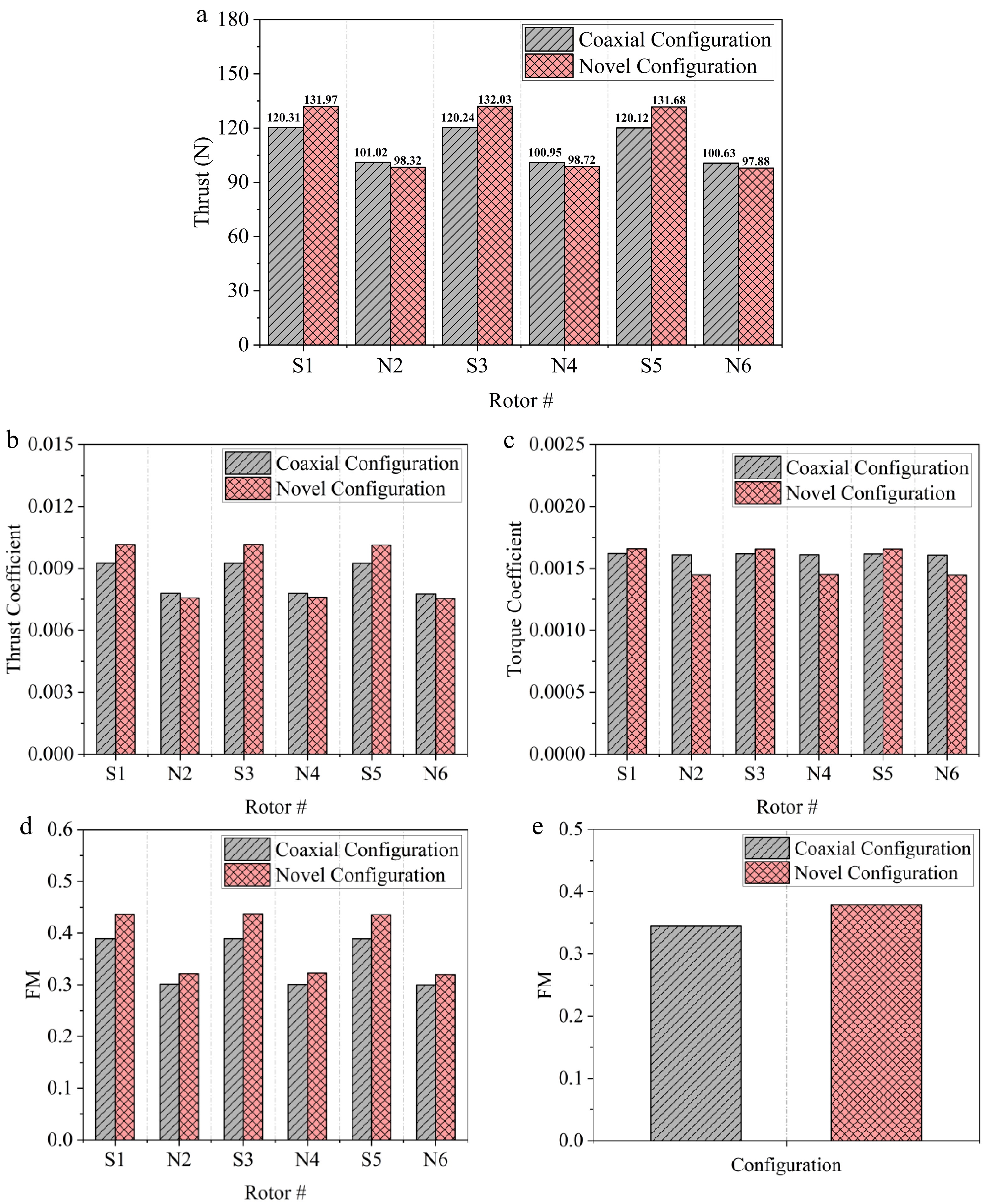
Figure 10.
Aerodynamic performance of three large-sized rotors. (a) Rotor thrust. (b) Thrust coefficient. (c) Torque coefficient. (d) FM of each rotor. (e) Average FM of the hexacopter.
-
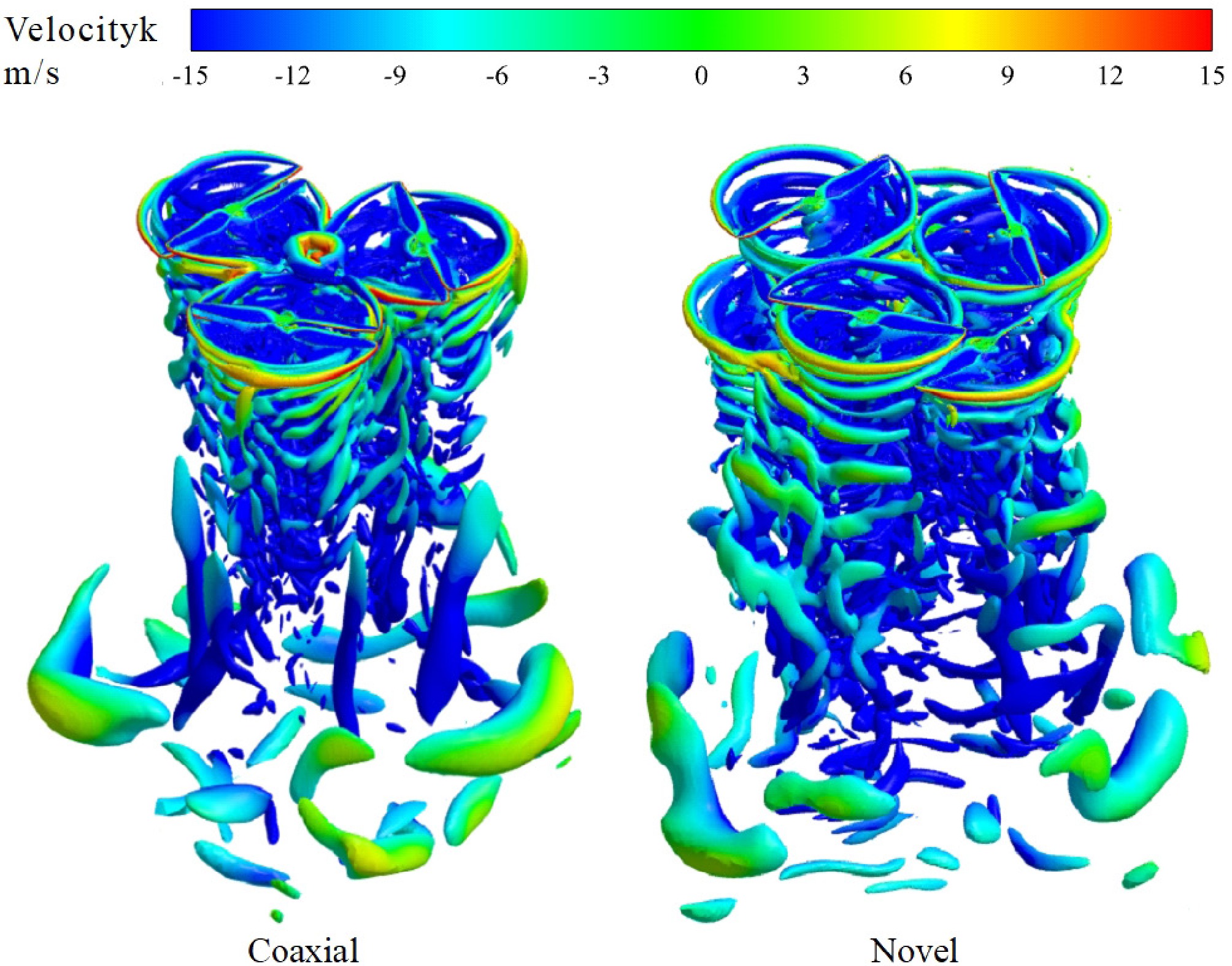
Figure 11.
Isosurface of Q-criterion and z-velocity for large-size rotors.
-
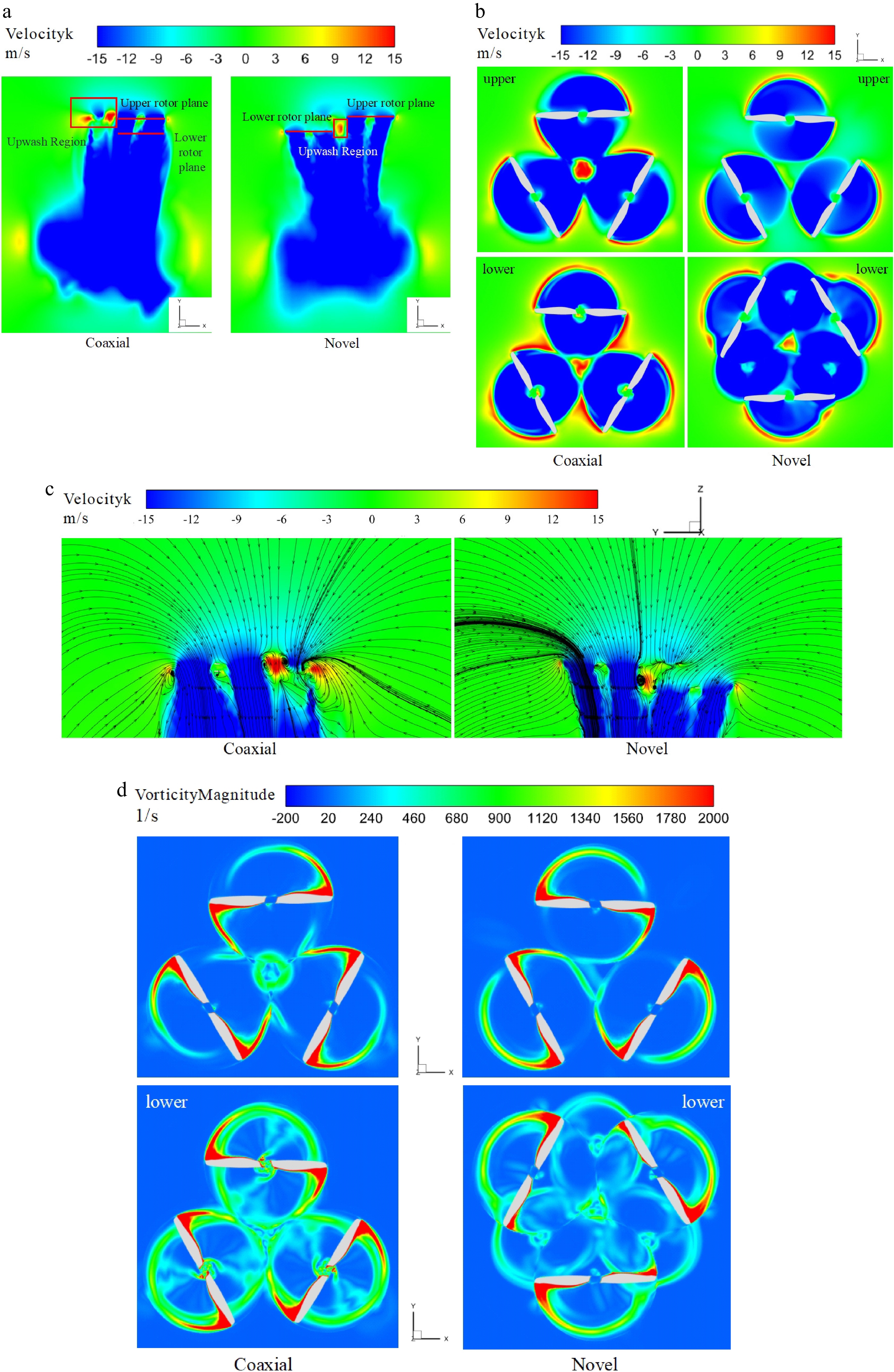
Figure 12.
(a) Downwash velocity distributions; (b) z-velocity at the rotor disk plane; (c) z-velocity-streamline distributions; (d) vorticity distributions at the rotor disk plane.
-
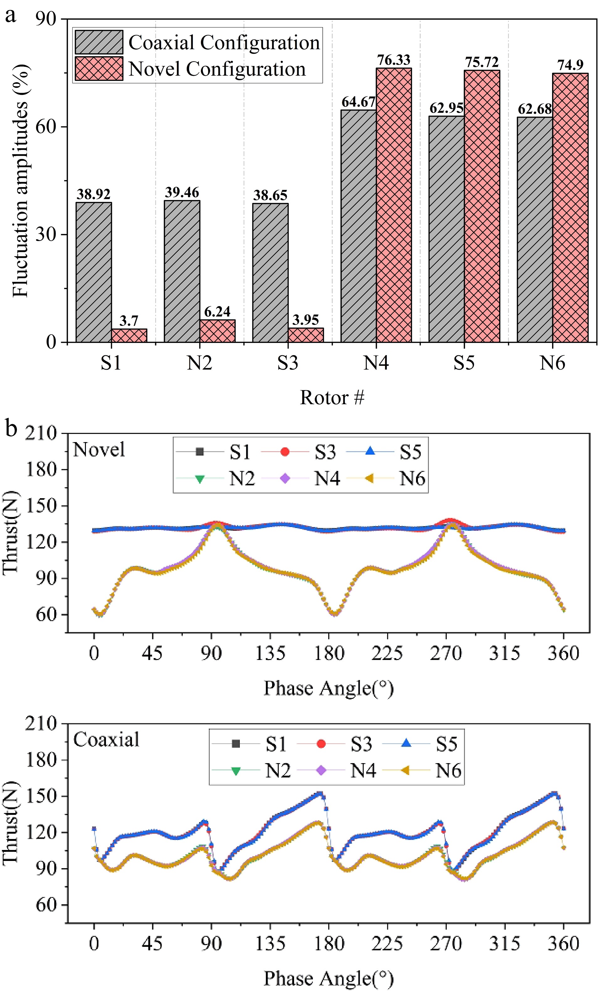
Figure 13.
(a) Ratios of peak-to-trough fluctuation amplitudes of instantaneous thrust to mean thrust; (b) thrust variation with phase during one revolution.
-
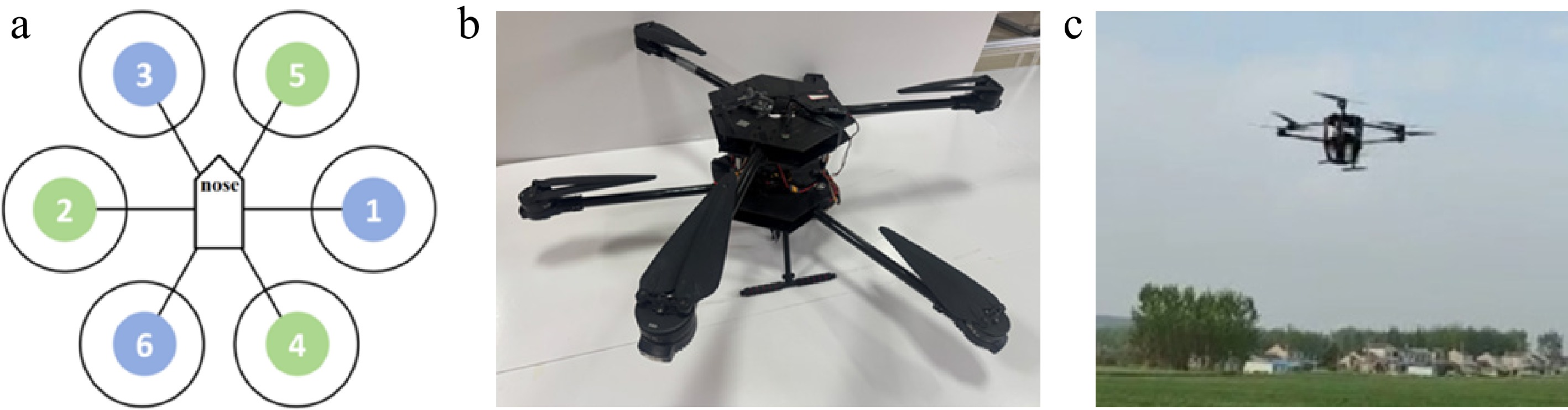
Figure 14.
(a) 'X' layout control scheme; (b) prototype of the novel hexacopter configuration; (c) flight test.
-
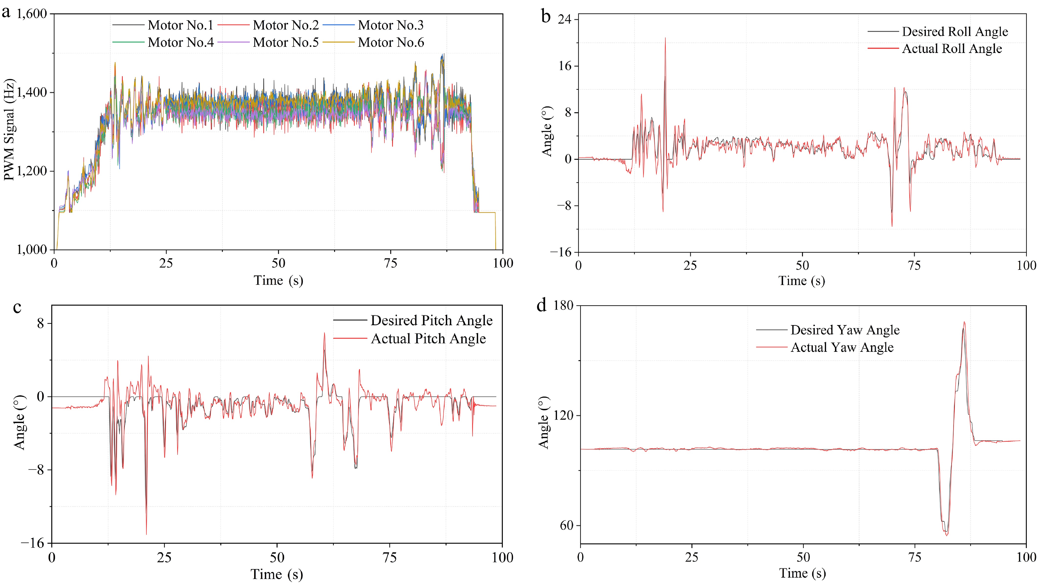
Figure 15.
(a) PWM signals of six motors over time; (b) time history of roll angle; (c) time history of pitch angle; (d) time history of yaw angle.
-
Experiment Simulation Relative error (%) CT-isolated rotor (10−2) 1.142 1.076 5.78 CQ-isolated rotor (10−3) 1.754 1.7938 2.27 Table 1.
Comparison of simulation and experimental results.
-
Rotational speeds 157.1 rad/s 209.4 rad/s 261.8 rad/s 314.2 rad/s 366.5 rad/s Number of grids Medium grids CT (10−2) 1.065 1.073 1.069 1.076 1.086 Rotor domain: 1.72 × 10⁶; Stationary domain 2.05 × 10⁶ Fine grids CT (10−2) 1.060 1.075 1.079 1.076 1.092 Rotor domain: 3.49 × 10⁶; Stationary domain 5.24 × 10⁶ Relative error (%) 0.472 0.186 0.927 0 0.549 / Medium grids CQ (10−3) 1.745 1.755 1.759 1.794 1.835 / Fine grids CQ (10−3) 1.682 1.701 1.712 1.749 1.754 / Relative error (%) 3.746 3.175 2.745 2.573 4.618 / Table 2.
Calculated results at different rotational speeds of the single rotor.
-
Rotor # S1 S3 S5 N2 N4 N6 Number of grids Medium grids CT (10−2) 1.059 1.059 1.058 1.064 1.065 1.065 Rotor domain: 1.19 × 10⁷; Stationary domain: 4.02 × 10⁶ Fine grids CT (10−2) 1.081 1.082 1.082 1.089 1.089 1.087 Rotor domain: 2.14 × 10⁷; Stationary domain: 5.24 × 10⁶ Relative error (%) 2.035 2.126 2.218 2.296 2.204 2.024 Medium grids CQ (10−3) 1.843 1.850 1.843 1.862 1.867 1.869 Fine grids CQ (10−3) 1.787 1.786 1.779 1.789 1.801 1.803 Relative error (%) 3.134 3.583 3.598 4.081 3.665 3.661 Table 3.
Calculated results for each rotor of the complete hexacopter system.
Figures
(15)
Tables
(3)