-
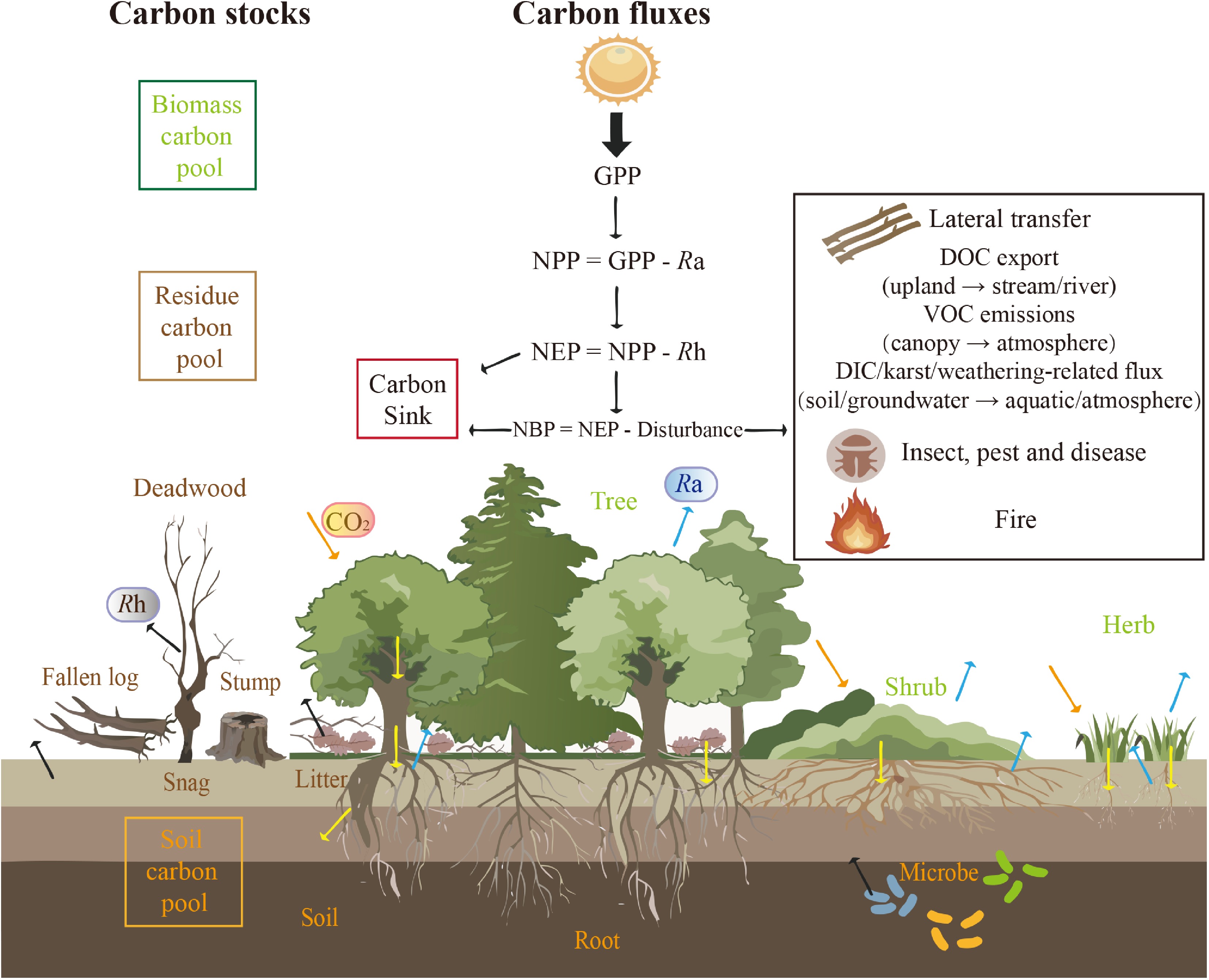
Figure 1.
Forest carbon cycle with key stocks, fluxes, and key pathways. Green indicates the biomass carbon pool (tree, shrub, herb), brown indicates the residue carbon pool (fallen log, stump, snag, litter), and orange indicates the soil carbon pool (soil, microbe). Arrows represent carbon-cycle processes: orange arrows indicate CO2 uptake through plant photosynthesis (GPP), yellow arrows indicate carbon transfer among pools (e.g., litterfall and root inputs), blue arrows denote autotrophic respiration (Ra), and black arrows denote heterotrophic respiration (Rh). Flux relationships are shown as NPP = GPP − Ra and NEP = NPP − Rh, while net biome productivity is expressed as NBP = NEP − D, where D represents disturbance-related carbon losses (e.g., fire, pests, harvest/windthrow). The figure also highlights non-vertical pathways such as DOC export, VOC emissions, and DIC/weathering-related fluxes that can influence ecosystem carbon balance.
-
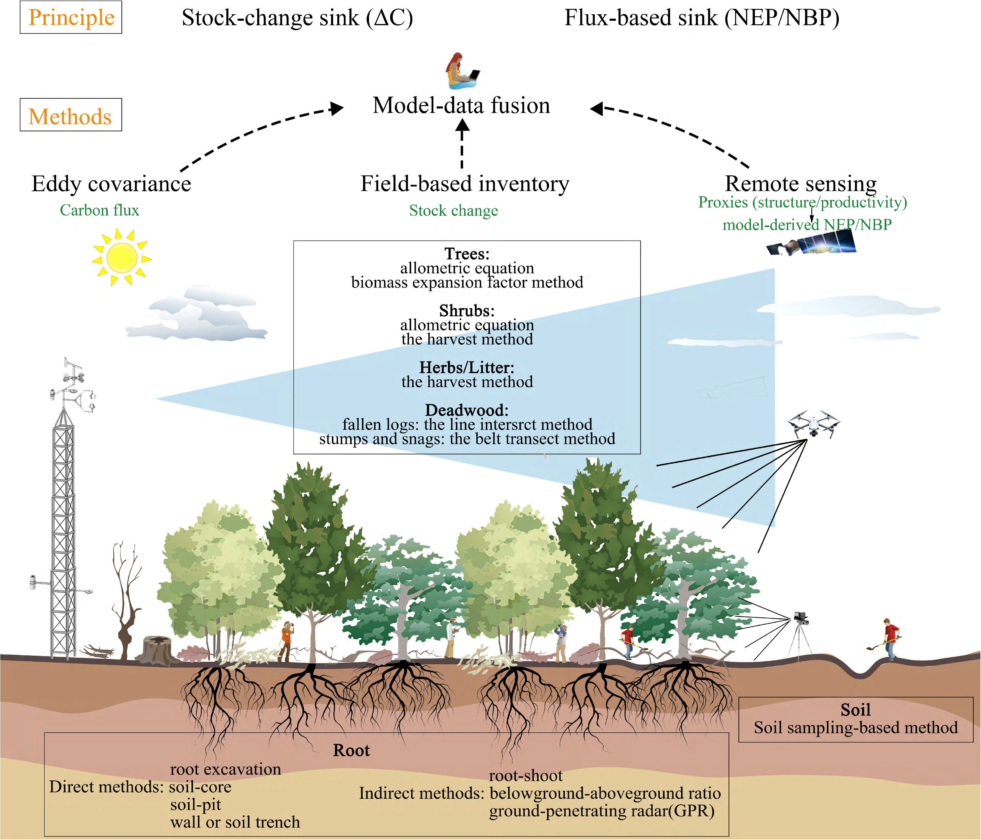
Figure 2.
Major approaches for estimating forest carbon sinks. Conceptual comparison of three method families: field-based inventory (stock-change, ΔC), eddy covariance (flux-based NEE/NEP), and remote sensing-model integration (structure/productivity proxies translated to model-derived NEP/NBP). The diagram emphasizes model-data fusion and cross-method complementarity for upscaling and interpretation.
-
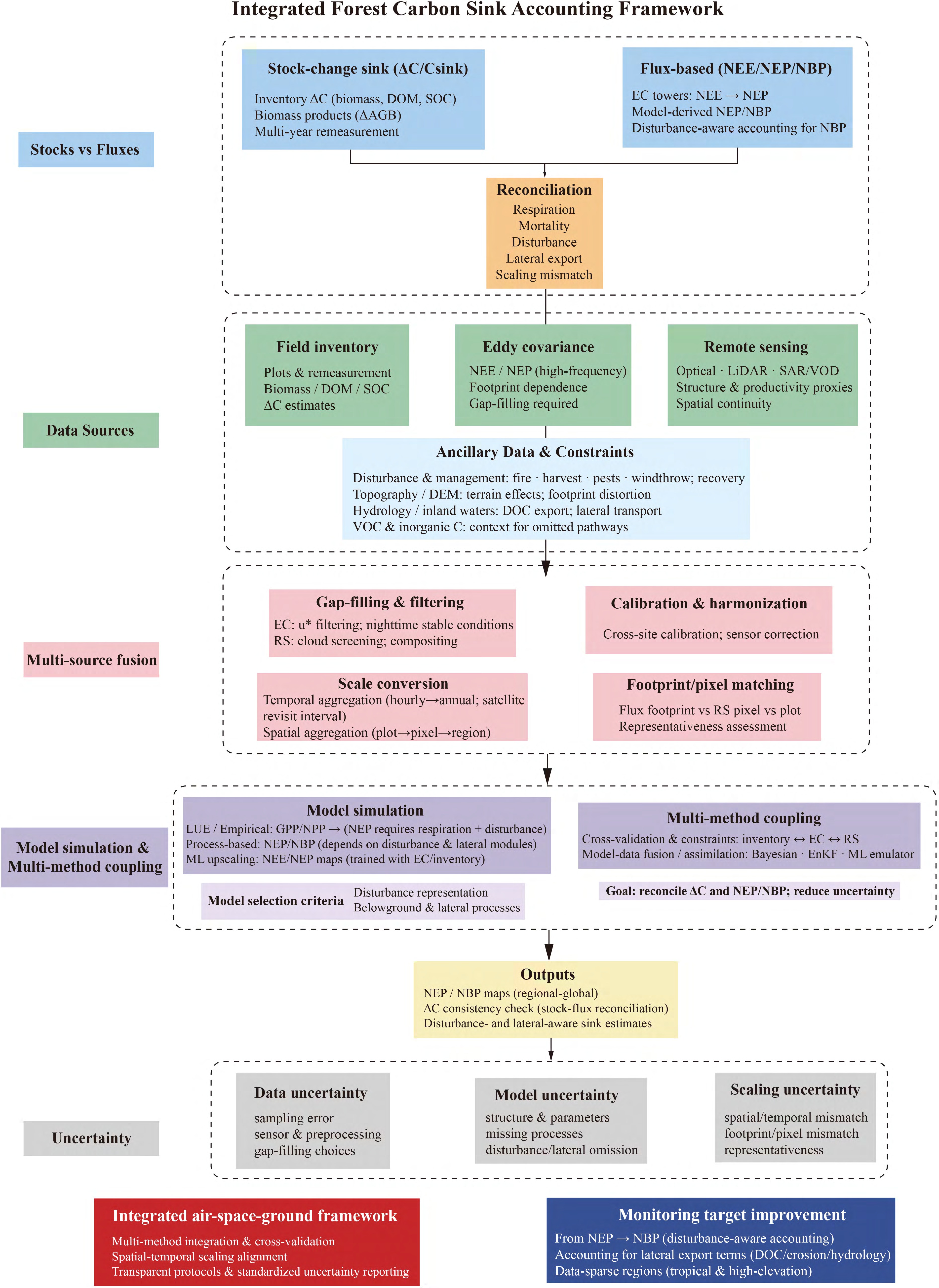
Figure 3.
Integrated framework for reconciling stock-change and flux-based sink estimates. Workflow linking ΔC/C_sink and NEE/NEP/NBP through a reconciliation step that considers respiration, mortality, disturbance, lateral export, and scaling mismatch. Inputs include inventory, eddy covariance, remote sensing, and ancillary constraints (disturbance/management, topography/DEM, hydrology/DOC, and VOC/inorganic-carbon context). The framework summarizes key fusion steps (gap-filling/filtering, calibration, scale conversion, footprint/pixel matching), model pathways, and uncertainty partitioning (data, model, scaling), and concludes with an air-space-ground monitoring strategy. Abbreviations: ΔC, change in ecosystem carbon stock; Csink, stock-change carbon sink estimated as ΔC per unit time; NEE, net ecosystem exchange; NEP, net ecosystem productivity; NBP, net biome productivity; EC, eddy covariance; DOM, dead organic matter; SOC, soil organic carbon; ΔAGB, change in aboveground biomass; DEM, digital elevation model; DOC, dissolved organic carbon; VOC, volatile organic compounds; u*, friction velocity threshold used for EC quality filtering; RS, remote sensing; LiDAR, Light Detection and Ranging; SAR, synthetic aperture radar; VOD, vegetation optical depth; LUE, light-use efficiency; GPP, gross primary productivity; NPP, net primary productivity; ML, machine learning; EnKF, Ensemble Kalman Filter.
-
Method Field-based inventory Eddy covariance Remote sensing Concept Stock-change accounting (ΔC) from repeated measurements of ecosystem carbon pools (AGB/DOM/SOC) using allometry/BEF Real-time measurement of CO2 fluxes in forest ecosystems by an in situ eddy covariance system Satellite observations provide structure/productivity proxies; NEP/NBP is inferred via models Temporal resolution of measured data Repeated pool measurements at multi-year intervals (typically 5–10 years) High-frequency flux measurements (typically 10–30 Hz, commonly stored as 30-min aggregates) Sensor revisit intervals from days to weeks; annual products typically derived after compositing/model integration Sampling Discrete point sampling Tower-based flux footprint (variable source area depending on wind and stability) Areal continuous observation Resources High labor and time costs High instrument and maintenance costs Data access, preprocessing, and substantial computing; requires ground/flux data for calibration/validation Model Allometric/BEF and stock-change accounting Flux processing and gap-filling, and partitioning Empirical/ML upscaling; LUE; process-based; data assimilation Advantage Long-term, policy-relevant stock accounting; spatially explicit pool estimates; robust for biomass trends when sampling and allometry are well calibrated Direct, continuous ecosystem-scale CO2 exchange (tower footprint) with high temporal resolution;
captures diurnal-interannual variabilityWide spatial coverage; repeated observations of canopy structure/condition; efficient regional-to-global mapping; long time-series availability (sensor dependent) Limitation Coarse temporal resolution;
allometry/BEF and sampling bias;
high uncertainty in SOC/belowground pools; disturbance/harvest attribution gaps;
ΔC-to-NEP/NBP conversion is assumption-rich and scale-dependentLow turbulence / stable stratification;
gap-filling/partitioning choices;
advection & complex terrain;
footprint representativenessCloud/saturation; sensor/preprocessing (atmospheric/geometric/terrain); indirect inference; model structural uncertainty;
scaling mismatchMain factors influencing uncertainty Sampling design, plot representativeness, allometric equations/BEF, belowground biomass, SOC heterogeneity, remeasurement interval Gap fraction, nighttime low turbulence,
u* filtering, gap-filling, flux partitioning, advection, terrain complexity, footprint representativenessCloud contamination, signal saturation, atmospheric/geometric/terrain correction, sensor type, calibration data, model structure, scaling mismatch Application Scale Tree-level
Stand-level
Regional scale
National scaletower footprint (~102–104 m radius; context dependent) network synthesis Stand-level
Regional scale
National scale
Global scalePrimary observed variable ΔC in pools (AGB/DOM/SOC) NEE (→NEP via sign convention; NBP requires disturbance/management losses) Structure/productivity proxies (AGB, LAI, fPAR, GPP/NPP) and model-derived NEP/NBP Table 1.
Comparative summary of major approaches for forest carbon sink estimation and key uncertainty characteristics.
-
Forest system Methods compared Variables compared Main finding relevant to this review Ref. Forest sites across boreal, temperate, and tropical zones Eddy covariance (EC) vs biometric methods (BM) Annual NEP, Reco, and GPP EC and BM produced different estimates of NEP, whereas Reco and GPP were generally more comparable. Methodological discrepancies were more pronounced in boreal forests, where net fluxes are smaller and source-sink classification is therefore more sensitive to methodological differences. [79] Coastal Douglas-fir stands, British Columbia, Canada Inventory-based stock change, EC-flux-tower estimates, and CBM-CFS3 model estimates ΔC and cumulative ΣNEP Cross-method comparison required explicit matching of inventory measurements, tower-based fluxes, and model estimates over comparable periods. The study showed that interpretation of agreement among methods depends strongly on topography, disturbance history, stand structure, and footprint-weighted comparison between tower fluxes and inventory plots. [49] Table 2.
Representative studies for cross-method comparison of forest carbon sink estimates.
Figures
(3)
Tables
(2)