-

Figure 1.
Schematic diagram of satellite-MAV cooperative observation.
-
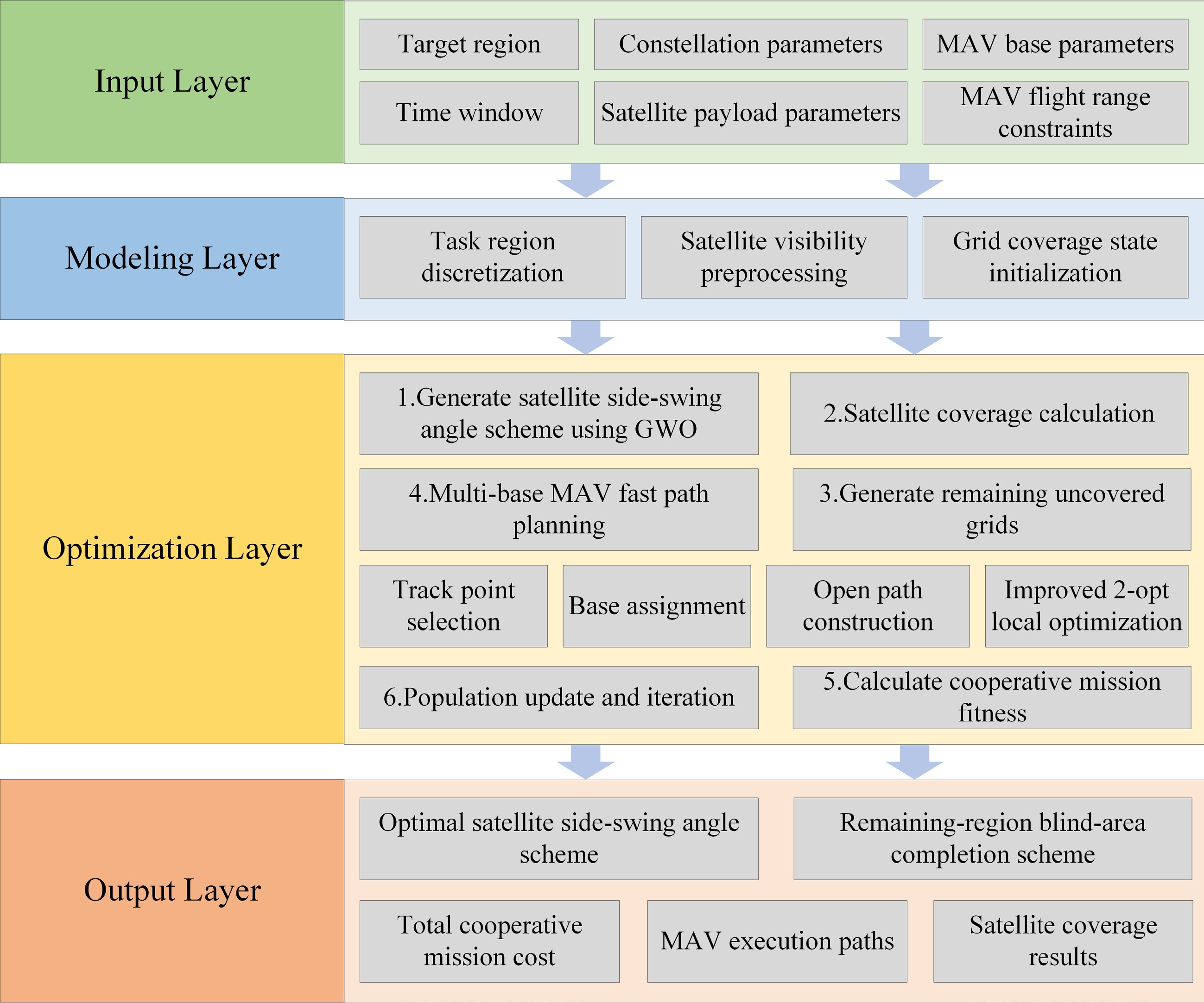
Figure 2.
Overall framework of the proposed GW-SWCRI method.
-

Figure 3.
Algorithm flow of MBM-FPP.
-
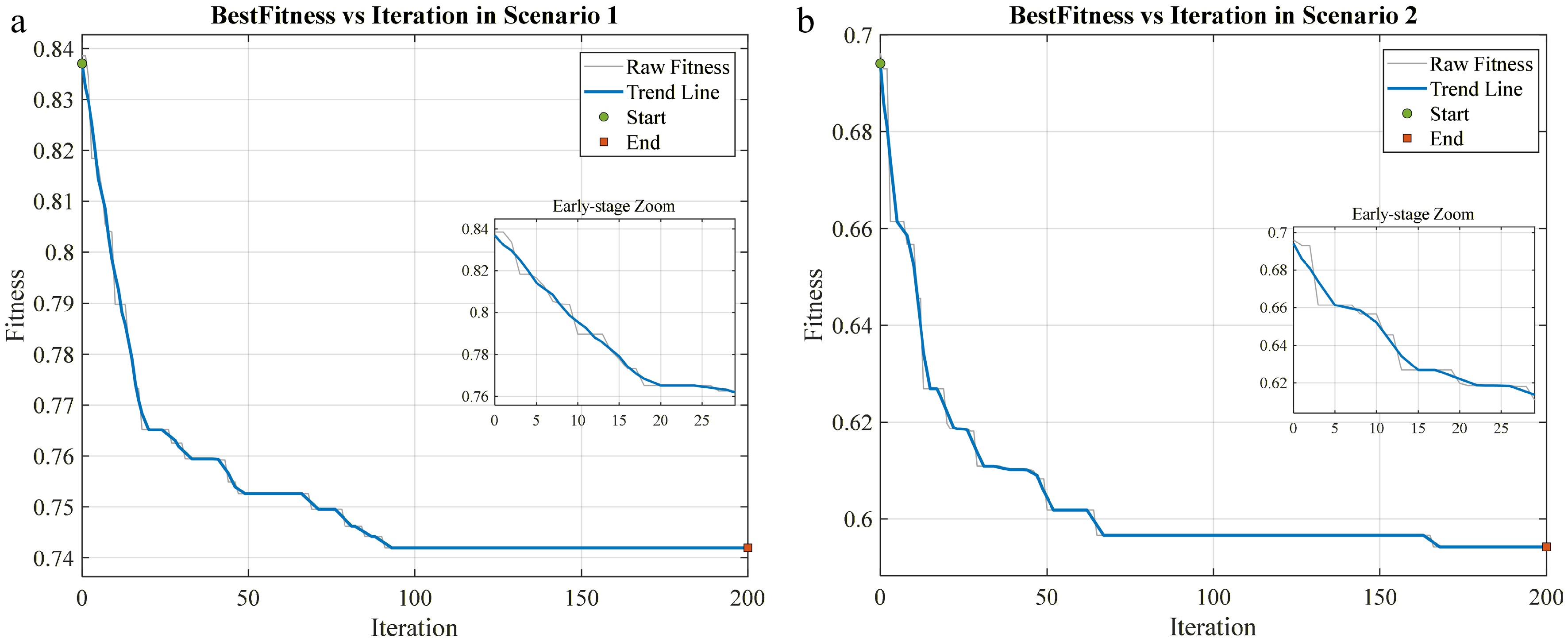
Figure 4.
Fitness value variation with iterations.
-
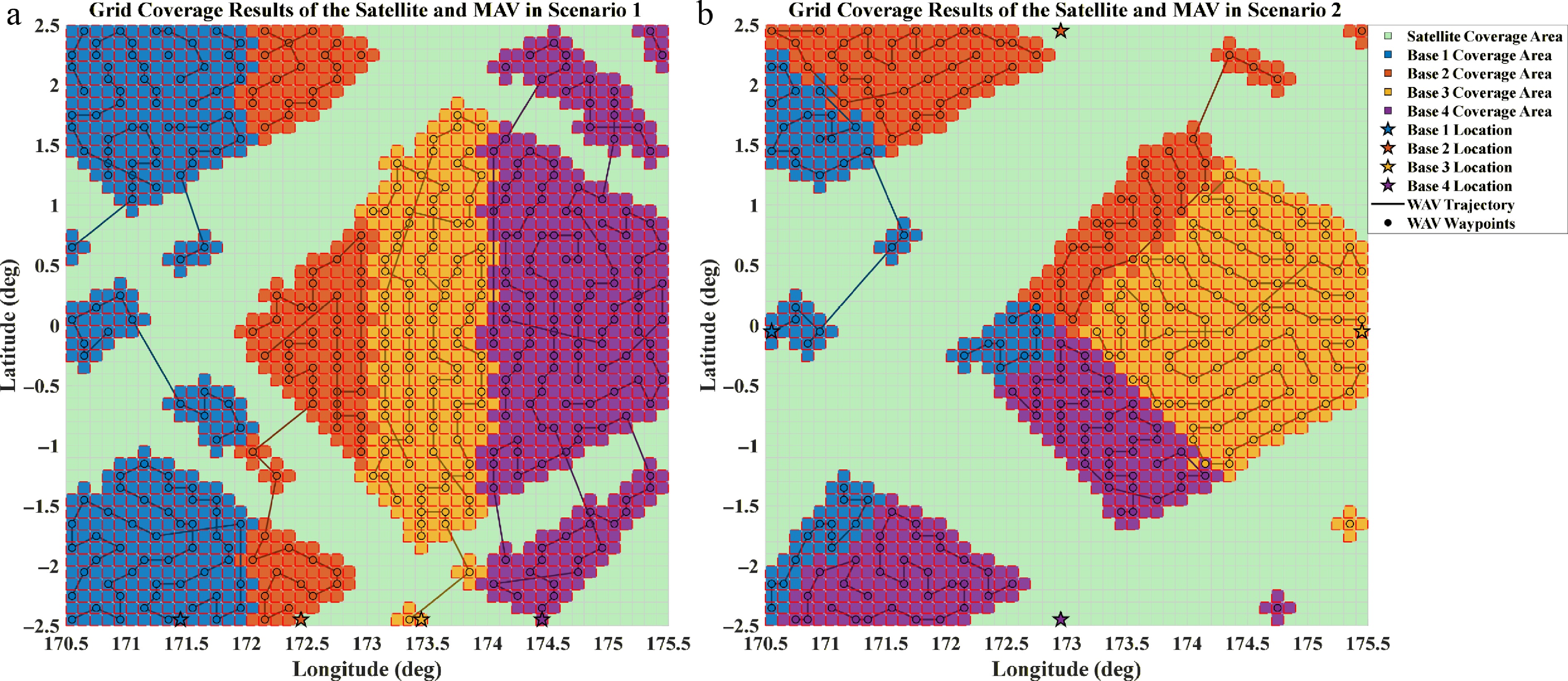
Figure 5.
Satellite and MAV grid coverage results.
-

Figure 6.
Variation of fitness value with iterations.
-
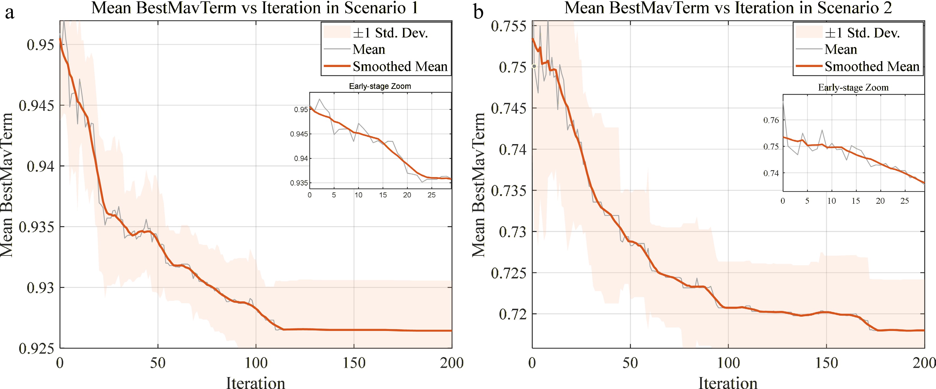
Figure 7.
Average optimal MAV cost term vs iteration number.
-
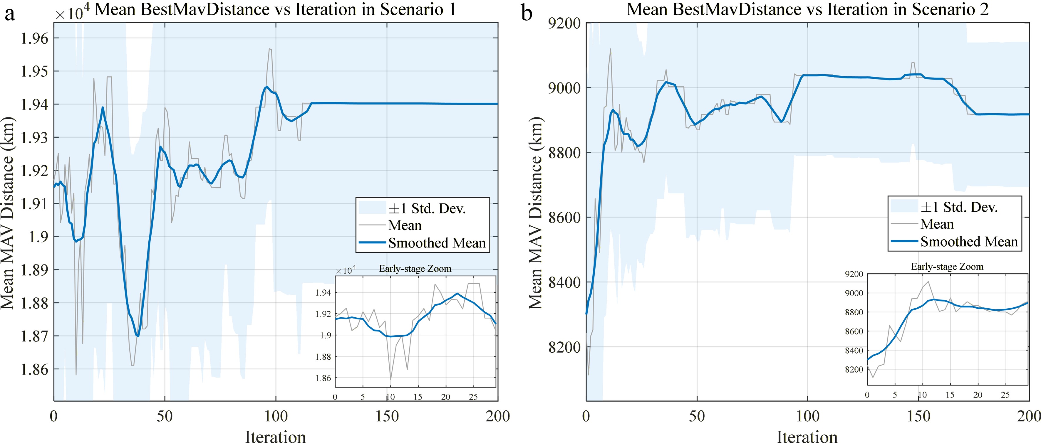
Figure 8.
Curve of average optimal MAV distance vs iteration number.
-
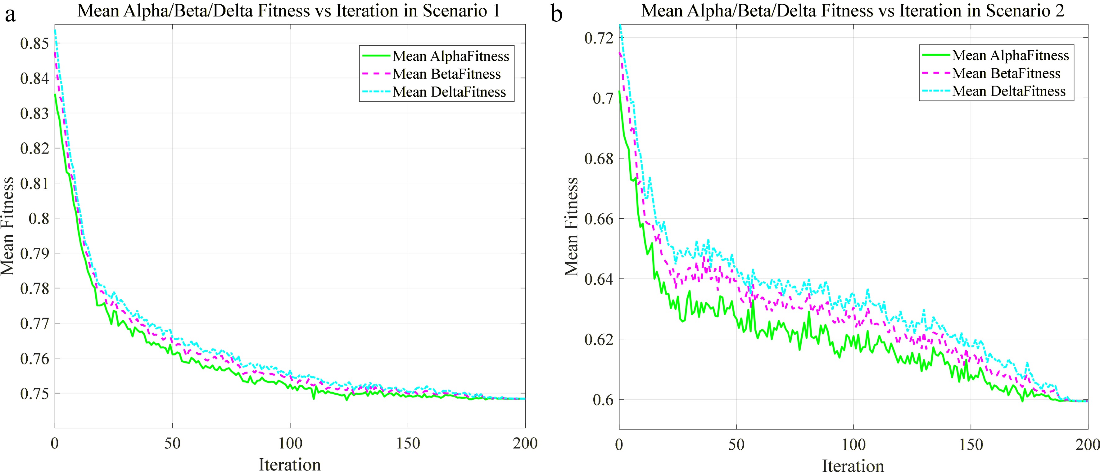
Figure 9.
Variation of fitness of the three leader wolves with iterations.
-

Figure 10.
Fitness variation curves with iterations for different algorithms.
-
Input: task region $ \Omega $ $ S $ $ B $ $ [At{t}_{\min },At{t}_{\max }] $ $ {D}_{\max } $ Output: optimal off-nadir angle code $ {b}^{*} $ $ R $ Initialize grey wolf population $ W $ Evaluate fitness and select $ \alpha $ $ \beta $ $ \delta $ for iteration t = 1 to $ {T}_{\max } $ for wolf $ {w}_{i} $ $ W $ Generate candidate position by GWO Limit step size and apply reflective boundary handling Update $ {w}_{i} $ end for Recalculate fitness and update $ \alpha $ $ \beta $ $ \delta $ end for $ {b}^{*} $ $ \alpha $ $ {g}_{unc} $ $ {b}^{*} $ $ {V}_{cand} $ $ {g}_{unc} $ Compute score $ F\left(v\right) $ $ v $ $ {V}_{cand} $ $ V $ $ F\left(v\right) $ Assign $ V $ for base $ {B}_{m} $ $ B $ while assigned waypoints are not empty do Initialize path $ r $ $ {B}_{m} $ while feasible waypoint exists do Select $ {v}^{*} $ $ G\left(v\right) $ Add $ {v}^{*} $ $ r $ end while Add $ r $ $ R $ end while end for for path $ r $ $ R $ Optimize $ r $ end for return $ {b}^{*} $ $ R $ Table 1.
Overall procedure of the GW-SWCRI method.
-
Constellation name Orbital altitude (km) Inclination (deg) Number of orbital planes Number of satellites per plane Phasing parameter Walker1 300 28.5 4 3 1 Walker2 300 45 4 5 1 Table 1.
Initial satellite parameters and constellation composition.
-
Scenario ID Cross-track pointing range (deg) Swath width (km) Imaging half-angle (deg) 1 [−30, 30] 60 5.711 2 [−15, 15] 90 8.531 Table 2.
Payload parameters for Scenarios 1 and 2.
-
Scenario ID Base ID X coordinate Y coordinate 1 1-1 10 1 1 1-2 20 1 1 1-3 30 1 1 1-4 40 1 2 2-1 1 25 2 2-2 25 50 2 2-3 50 25 2 2-4 25 1 Table 3.
Distribution of MAV bases in Scenarios 1 and 2.
-
Parameter Value Coverage gain weight 1.0 Boundary/isolated grid gain weight 0.6 Connected component gain weight 0.5 Base distance cost weight 0.8 Distance cost weight 1.0 Turn penalty weight 0.35 Path length weight 1.0 Turn cost weight 0.25 Flight range safety margin ratio 0.05 Risk penalty threshold 0.85 Maximum number of 2-opt iterations 100 Flight range risk penalty weight 2.0 Table 4.
Initial parameters of the MBM-FPP method.
-
Algorithm name Total running time (s) Average running time per iteration (s) GA (population size 20) 1,840.7 9.20 GWO (population size 20) 1,920 9.60 GS (population size 20) 1,230.3 6.15 GA (population size 50) 4,969.9 24.85 Table 5.
Running time of different algorithms.
Figures
(10)
Tables
(6)