-
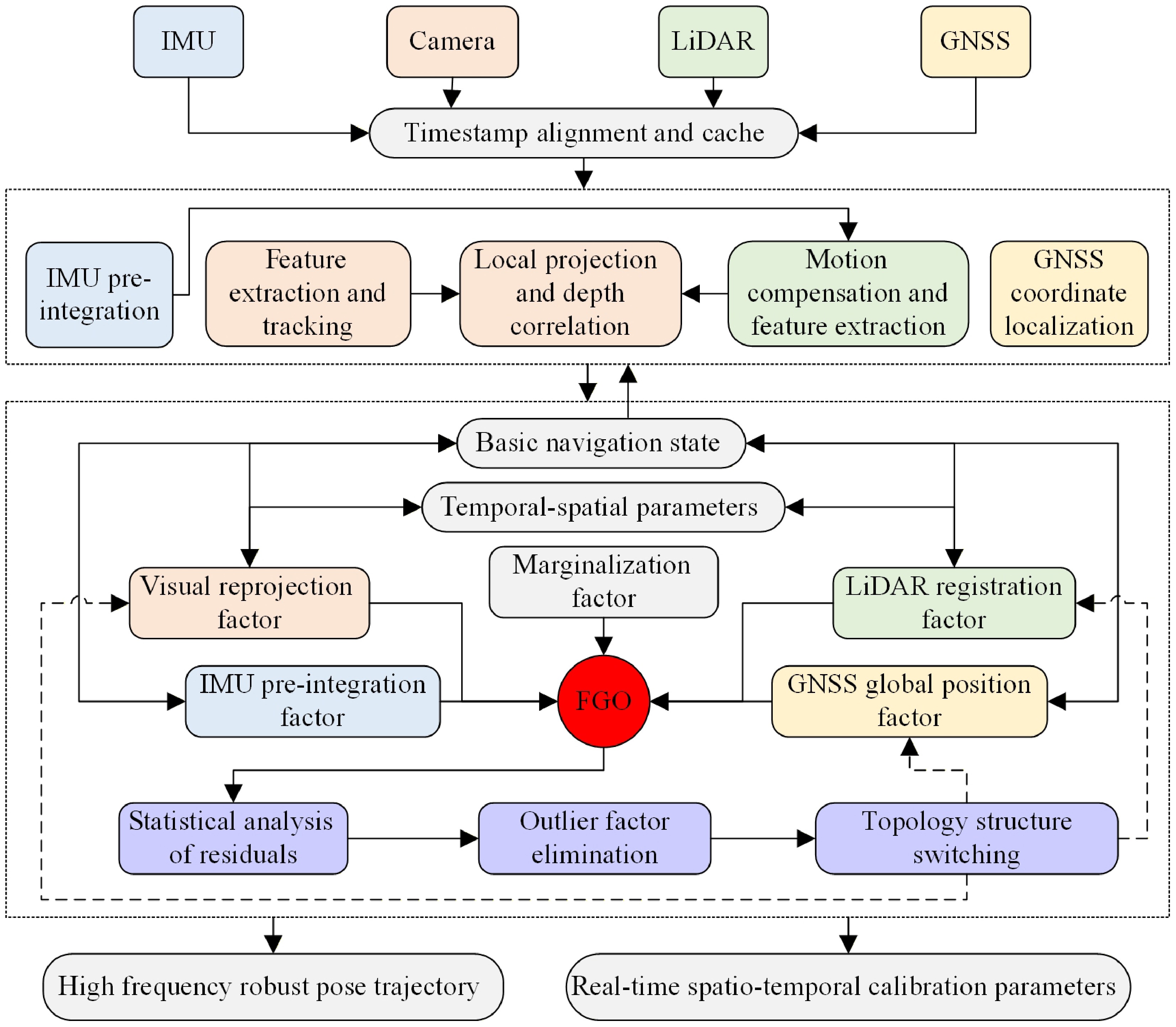
Figure 1.
Overview of elastic multi-source fusion navigation system.
-
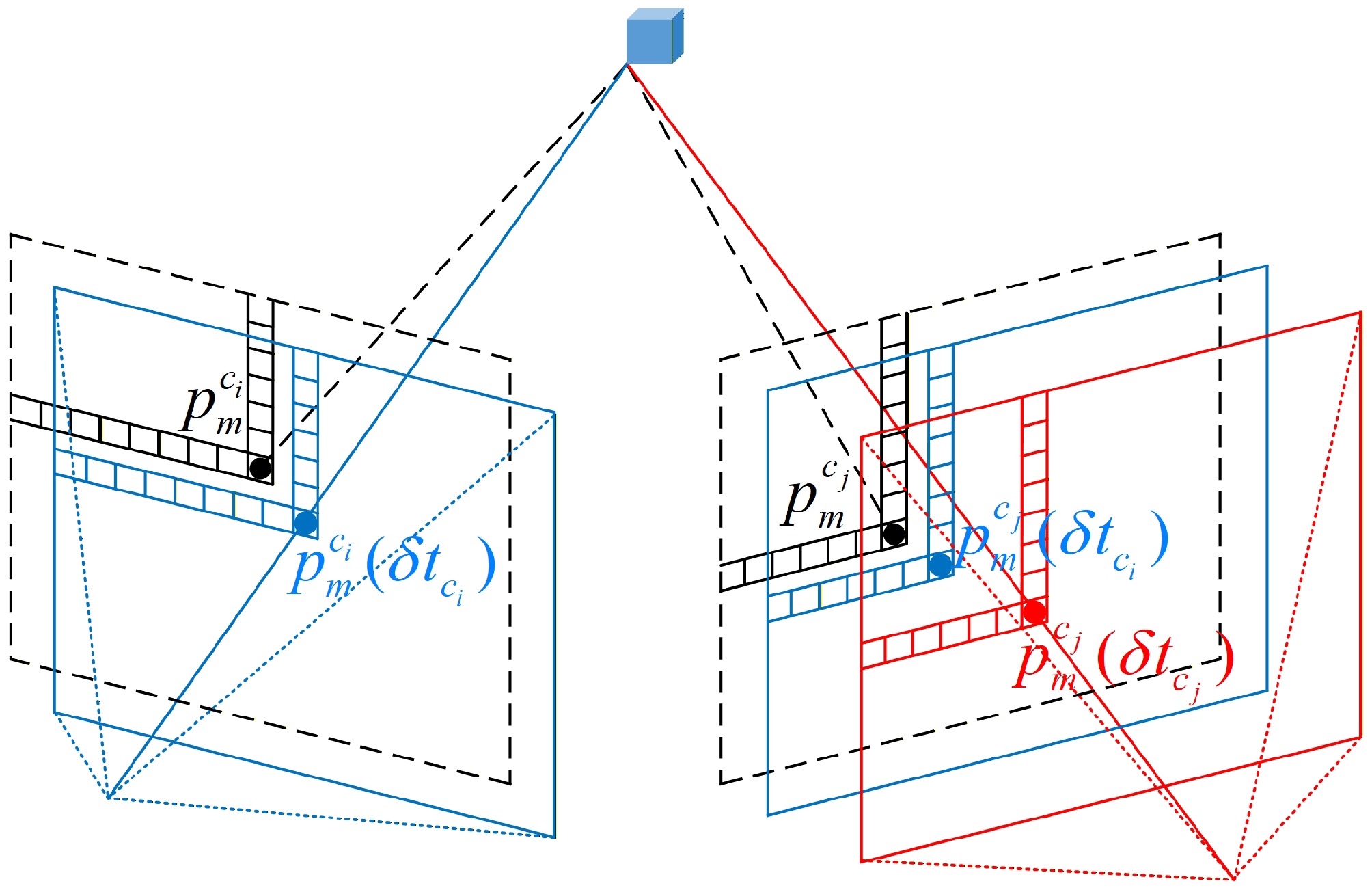
Figure 2.
Visual reprojection process considering time delay.
-
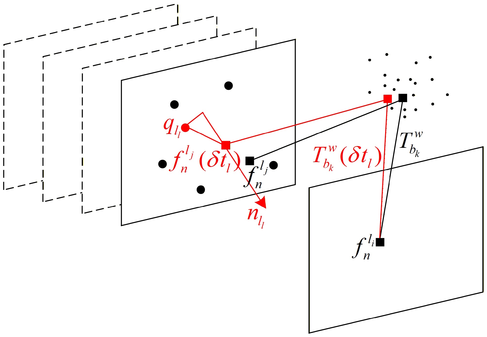
Figure 3.
LiDAR point cloud matching transformation considering time delay.
-
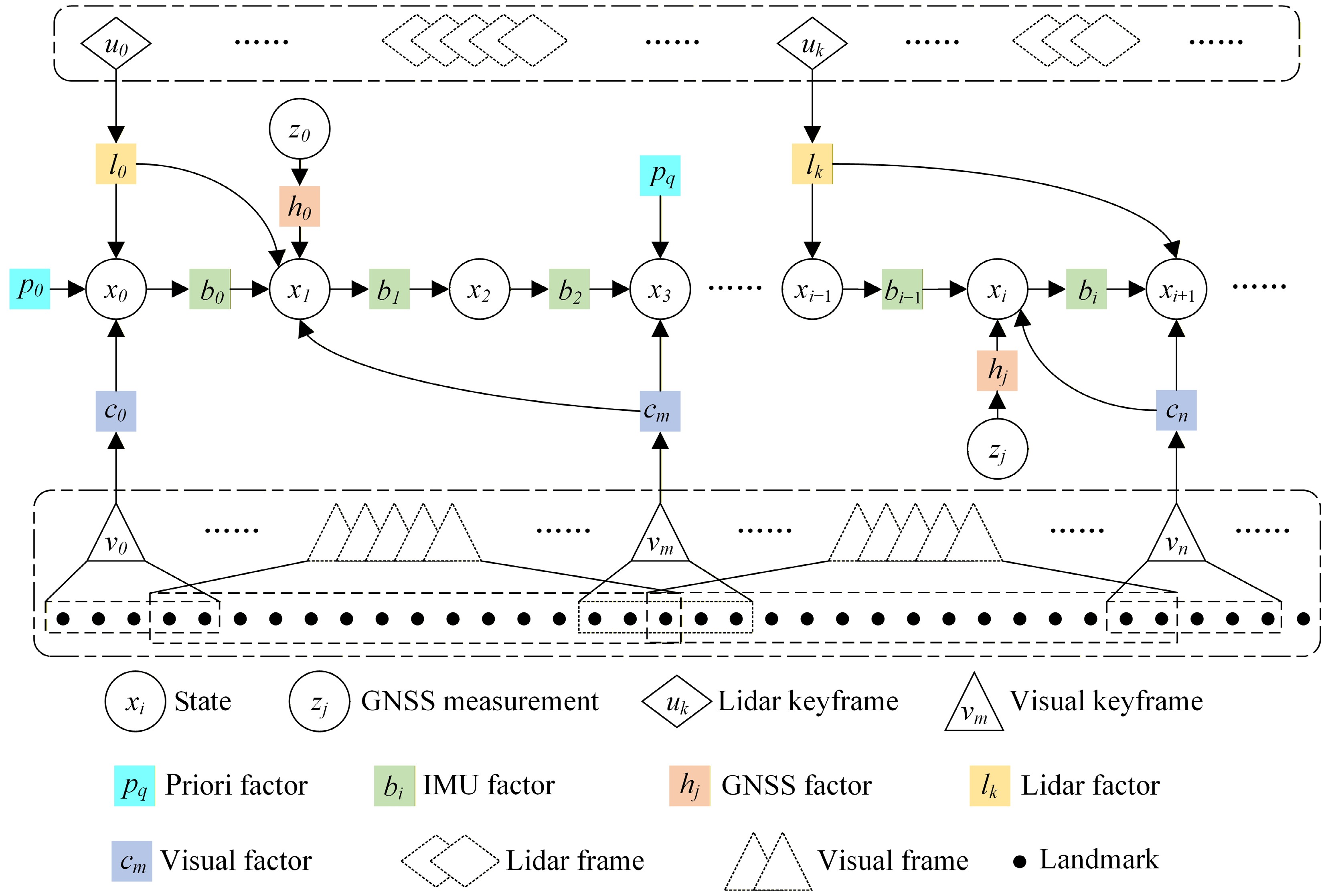
Figure 4.
Factor graph optimization framework.
-
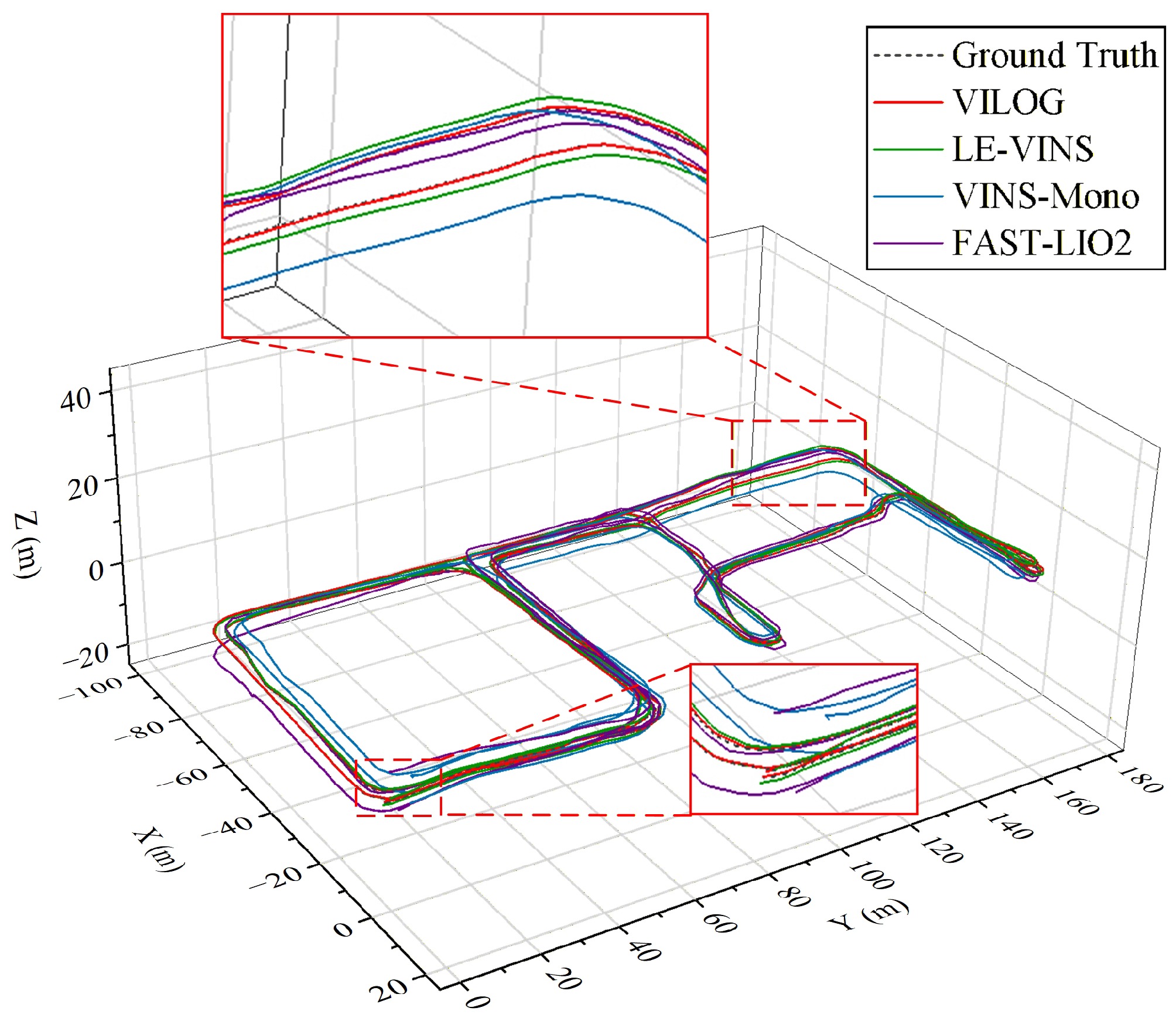
Figure 5.
Trajectory comparison of different algorithms.
-
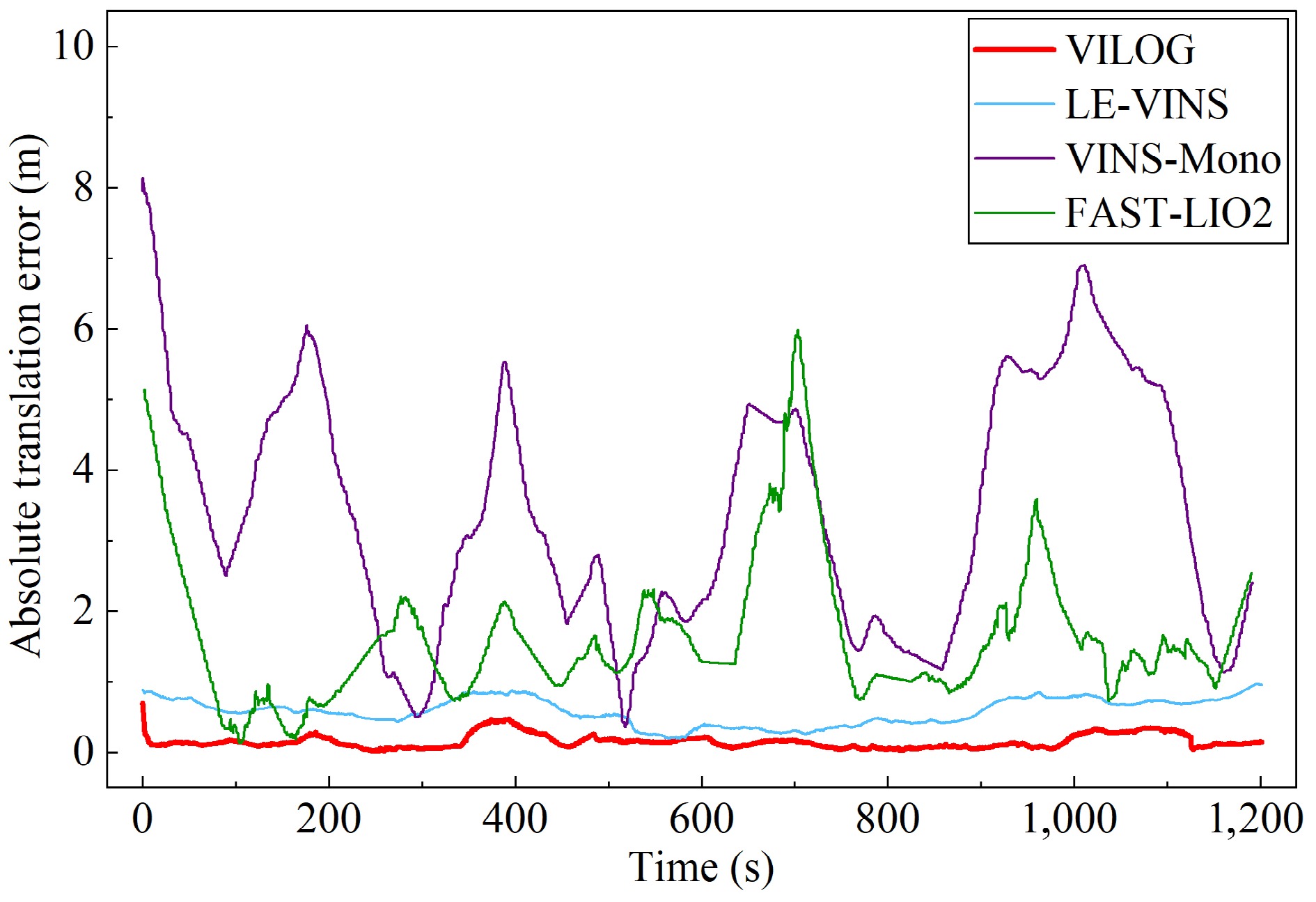
Figure 6.
ATE variation curve.
-
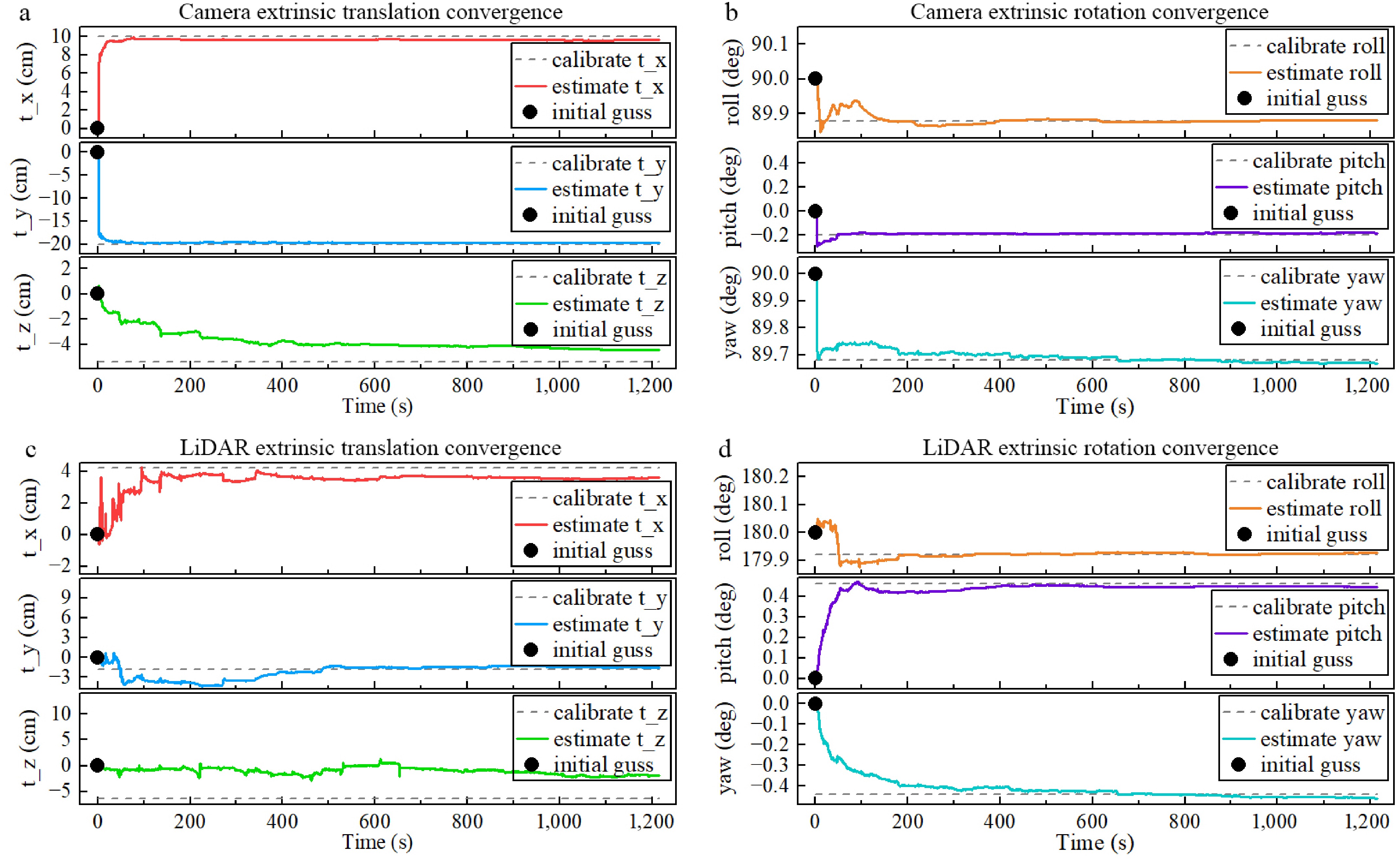
Figure 7.
Real-time calibration of camera and LiDAR extrinsic parameters.
-
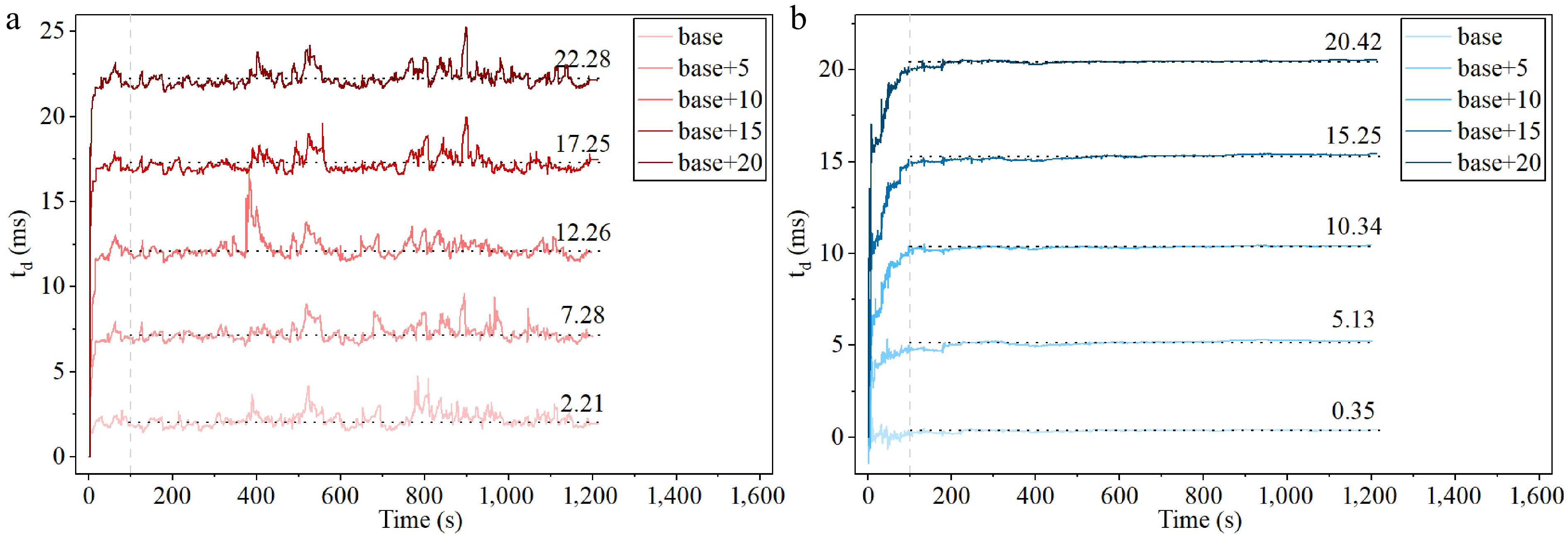
Figure 8.
Online estimation of camera-IMU and LiDAR-IMU temporal offsets.
-
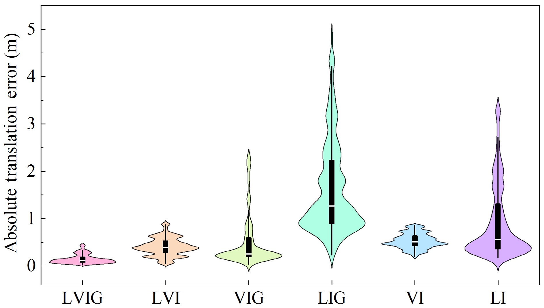
Figure 9.
ATE distribution of different sensor combinations.
-
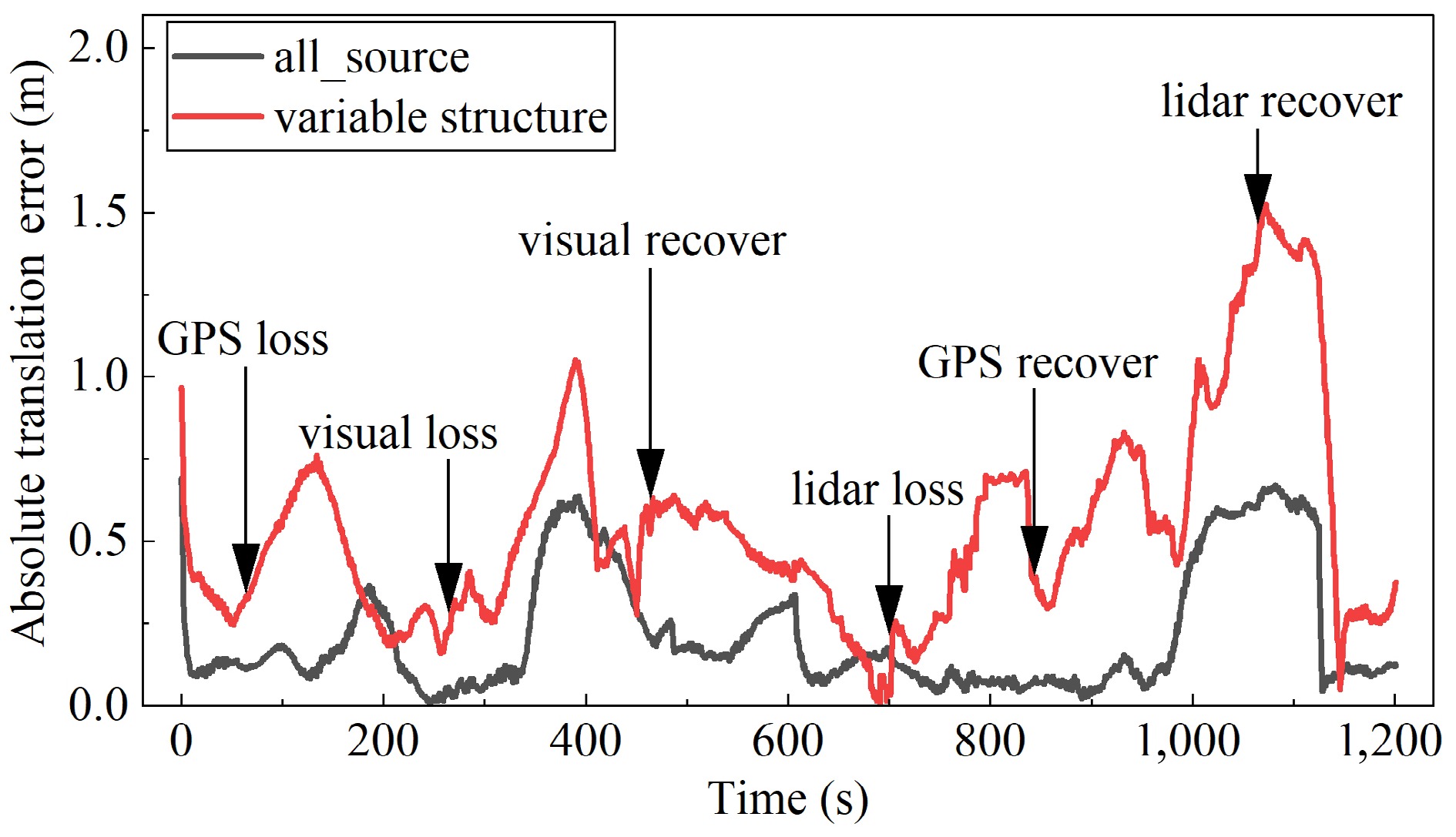
Figure 10.
ATE changes during sensor loss and recovery.
-
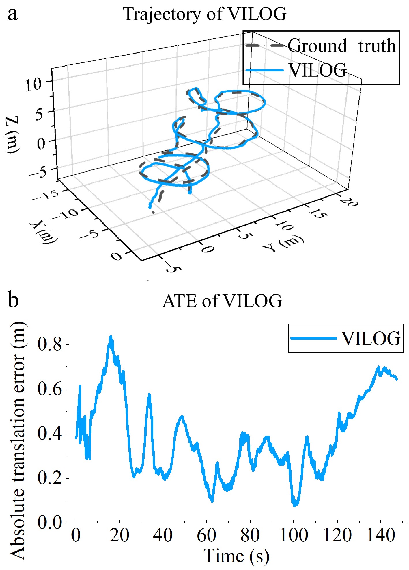
Figure 11.
Multi-source fusion navigation effect of MAV platform.
-
Input: sliding-window factors, initial states, marginalization prior Output: optimized states, calibration parameters, active topology 1: while a new sliding window is available do 2: Add parameters and residual blocks of IMU, GNSS, visual, LiDAR factors. 3: Perform the first LM optimization with N1 iterations. 4: for each factor bk from GNSS, visual, and LiDAR measurements do 5: Compute normalized squared residual $ \boldsymbol{\mathit{D}}_k=\boldsymbol{r}_k^T\boldsymbol{\Omega}_k\boldsymbol{r}_k $ 6: if $ \boldsymbol{\mathit{D}}_k \gt \chi_{0.99,v_k}^2 $ 7: Remove bk from the factor graph. 8: end if 9: end for 10: for each modality s $\in $ 11: Compute $ {\rho }_{s,i}=N_{s,i}^{removed}/N_{s,i}^{all} $ 12: if ρs,i > 50% then 13: Remove all factors of modality s in frame i and mark degraded. 14: end if 15: end for 16: Perform the second LM optimization with N2 iterations. 17: Update states and calibration parameters. 18: end while Table 1.
Elastic sliding-window optimization with chi-square factor culling.
-
Test algorithm ARE (deg) ATE (m) FAST-LIO2 3.04 1.90 VINS-Mono 0.67 3.82 LE-VINS 0.38 0.61 VILOG (ours) 0.21 0.18 Table 1.
Comparison data of different algorithms.
-
Increment set
(ms)Statistics of camera (ms) Statistics of LiDAR (ms) Mean Median RMSE Mean Median RMSE 5 5.08 5.05 0.43 4.79 4.81 0.24 10 10.05 10.01 0.52 10.00 10.01 0.05 15 15.04 15.04 0.43 14.90 14.93 0.14 20 20.07 20.04 0.44 20.08 20.08 0.11 Table 2.
Time offset increment estimation statistics.
Figures
(11)
Tables
(3)