-
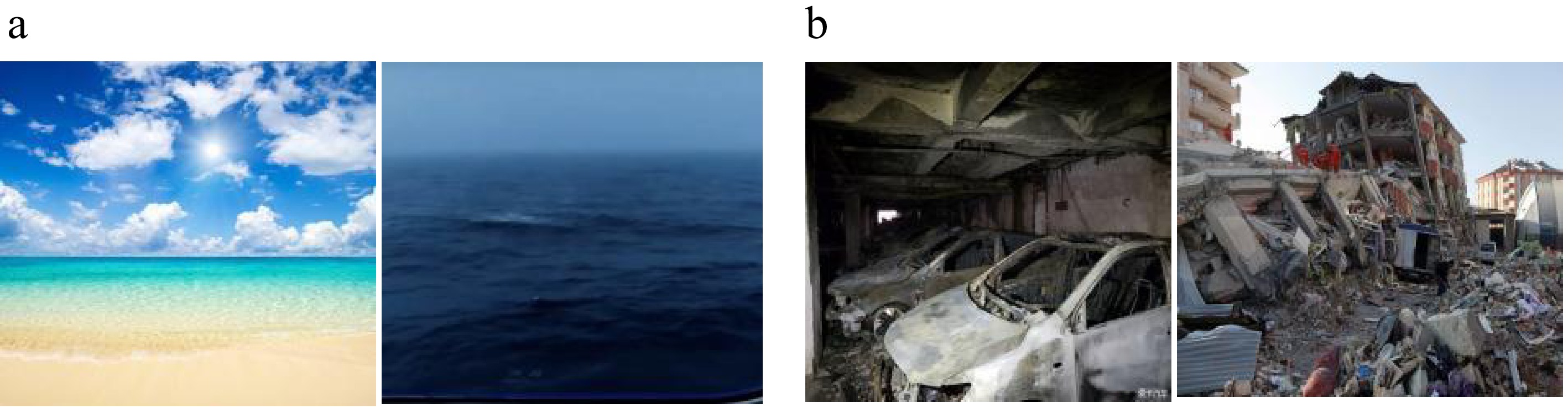
Figure 1.
Examples of the affective gap.
-
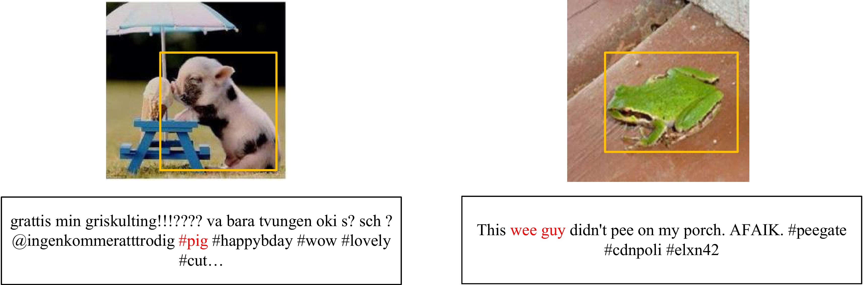
Figure 2.
Examples of image-text pairs collected from Twitter.
-
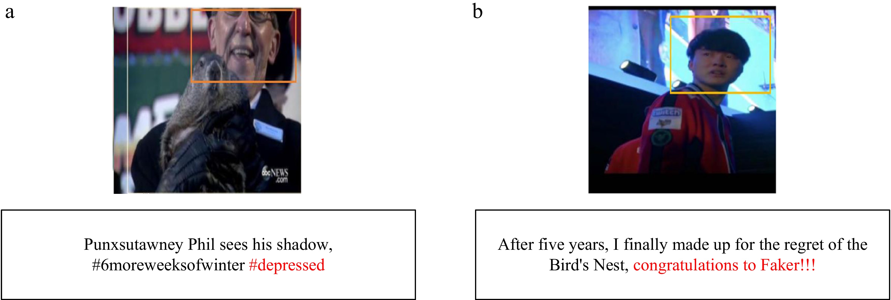
Figure 3.
Examples illustrating the unreliability of unimodal inference when text is dominated by subjective expressions or linguistic noise. The structured visual context provides the necessary semantic grounding for accurate sentiment prediction.
-
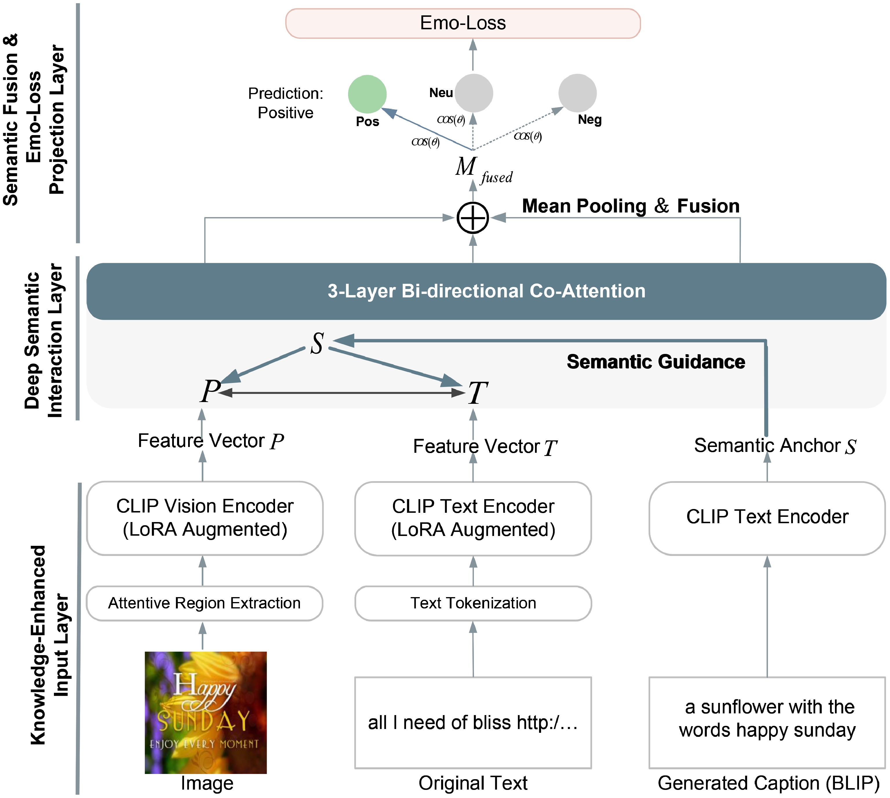
Figure 4.
The overall architecture of GSKA. The pipeline transitions from sensory encoding to knowledge-driven reasoning, culminating in an affective manifold mapping for sentiment prediction.
-
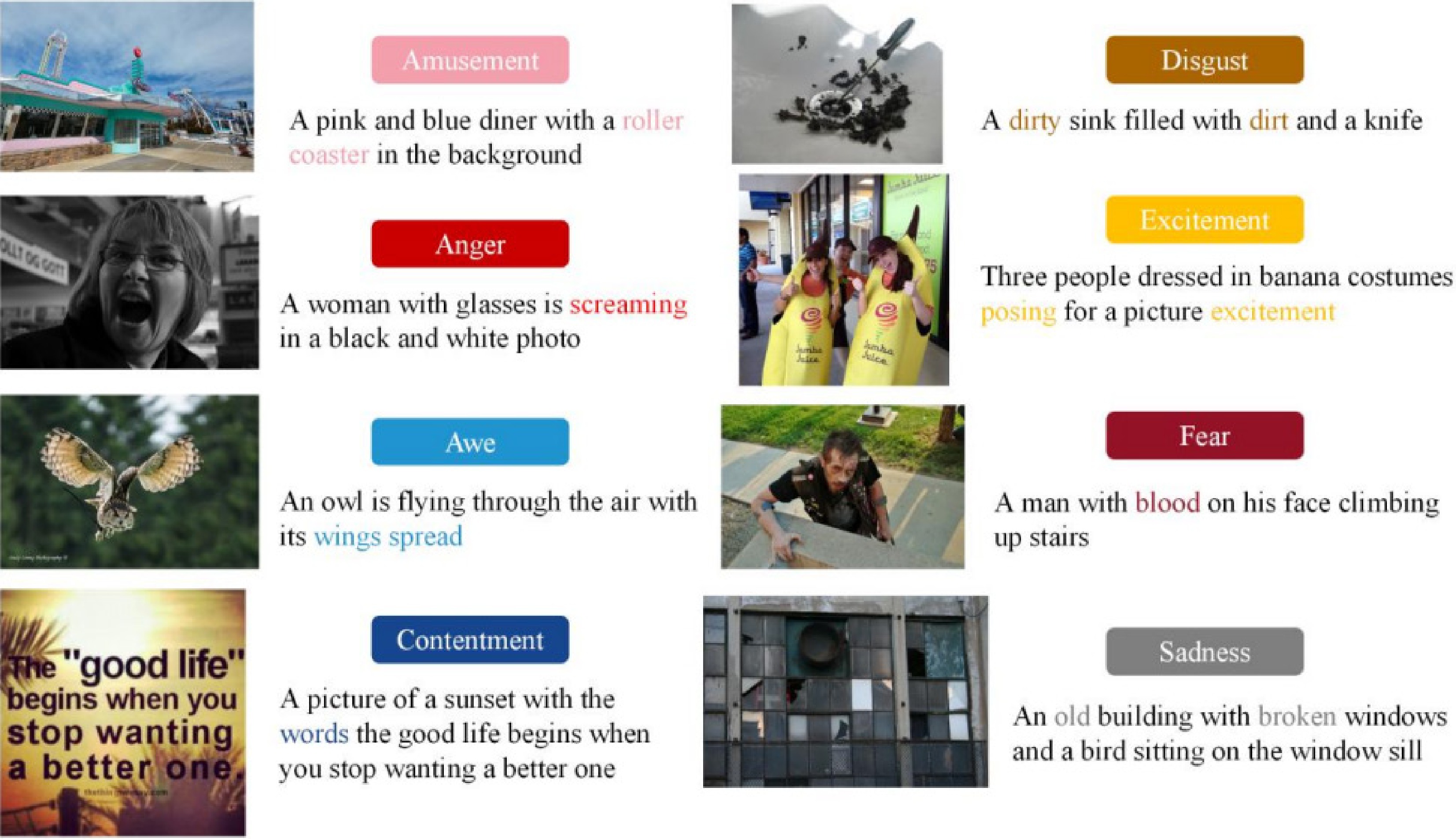
Figure 5.
Visualization of the generative semantic anchoring process. High-level affective indicators are extracted to serve as stable semantic coordinates (
$ {\bf{S}} $ -
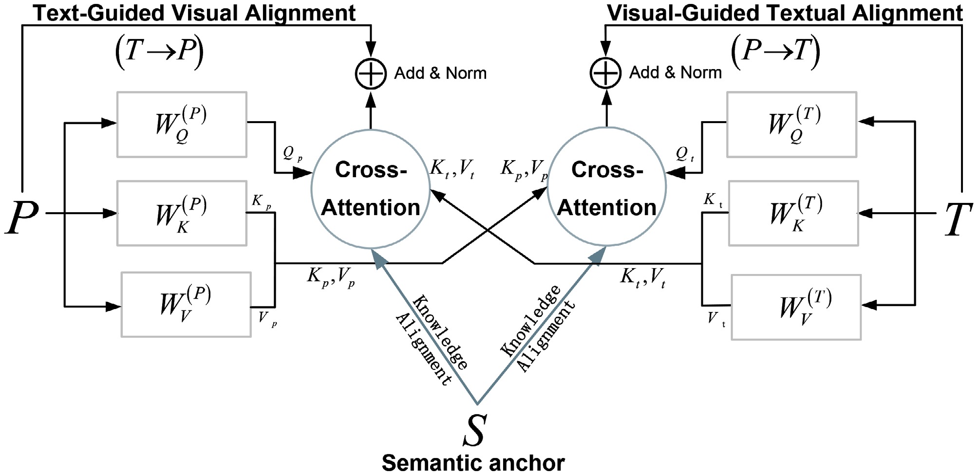
Figure 6.
Detailed mechanism of the Bi-directional Knowledge Alignment (BKA) module. The Semantic Anchor (
$ {\bf{S}} $ $ {\bf{P}} $ $ {\bf{T}} $ -
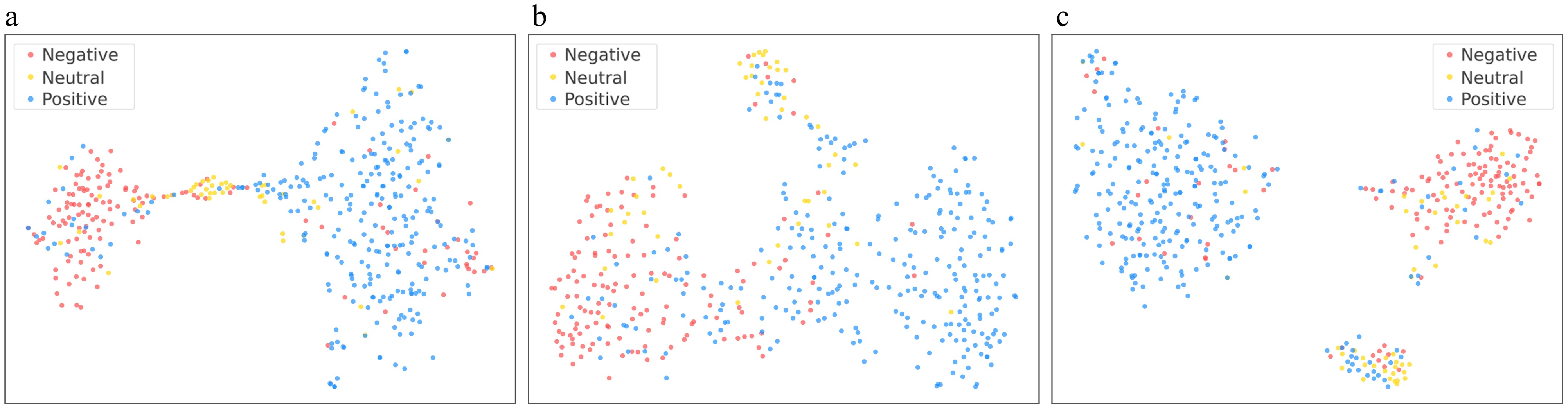
Figure 7.
t-SNE visualization of multimodal embeddings for different variants: (a) Standard Cross-Entropy; (b) Contrastive Loss; and (c) Emo-Loss (full GSKA).
-
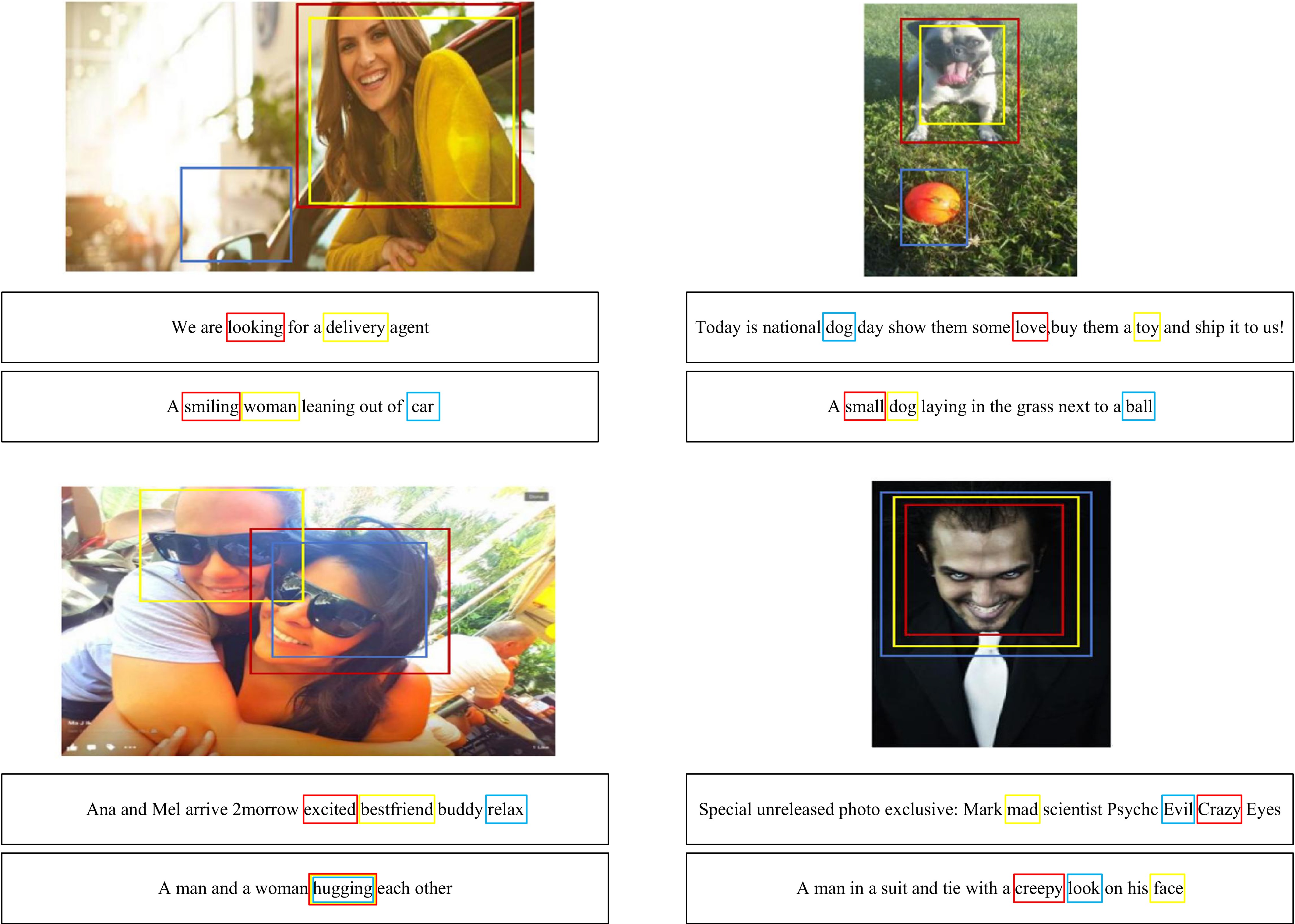
Figure 8.
Visualization of the attention mechanism, highlighting aligned image regions and textual tokens.
-
Input: Fused multi-modal feature $ M_{\text{fused}} $ $ y $ $ {\bf{C}} $ $ \beta $ Output: Emotional discrepancy loss $ {\cal{L}}_{Emo} $ 1. Similarity Calculation: Compute cosine similarities for all classes: $ s_j = {\text{cosine}}\_{\text{sim}}(M_{\text{fused}}, {\bf{c}}_j) $ $ j \in \{pos, neu, neg\} $ 2. Target Identification: Retrieve target similarity: $ s_{target} = s_y $ 3. Competitor Mining: Find maximum confounding similarity: $ s_{other} = \max_{j \neq y} (s_j) $ 4. Margin Optimization: Calculate similarity margin: $ \Delta = s_{target} - s_{other} $ 5. Non-linear Mapping: Normalize margin via scaled sigmoid: $ \text{diff} = 2 \cdot \sigma(\beta \cdot \Delta) - 1 $ 6. return $ {\cal{L}}_{Emo} = 1 - \text{diff} $ Table 1.
Emo-Loss computation.
-
Dataset Positive Neutral Negative Total MVSA-single 2,683 470 1,358 4,511 MVSA-multiple 11,318 4,408 1,298 17,024 Table 1.
Statistics of the datasets.
-
Modality Methods MVSA-single MVSA-multiple Accuracy F1 Accuracy F1 Text CNN 68.19 55.90 65.64 57.66 BERT 71.11 69.70 67.59 66.24 Image ResNet50 64.67 61.55 61.88 60.98 ViT 63.78 62.26 61.94 61.19 RepViT 64.82 62.81 62.01 61.35 TransNeXt 65.71 64.81 62.48 61.52 Multimodal HSAN 69.88 66.90 67.96 67.76 MultiSentiNet 69.84 69.63 68.86 68.11 Co-MN-Hop6 70.51 70.01 68.92 68.83 MVAN-M 72.98 72.98 72.36 72.30 MGNNS 73.77 72.70 72.49 69.34 CLMLF 75.33 73.46 72.00 69.83 MVCN 76.06 74.55 72.07 70.01 ICCI 79.33 77.51 73.29 70.06 MSFN 78.98 78.48 74.75 72.62 GSKA (ours) 80.93 80.10 75.05 74.57 Table 2.
Performance comparison on MVSA datasets. Accuracy and F1-score are reported as a percentage (%).
-
Variants Accuracy (%) $ \Delta $ F1 (%) $ \Delta $ GSKA (full model) 80.93 – 80.10 – w/o Co-Attention 77.42 $ \downarrow $ 76.88 $ \downarrow $ w/o Captioning 78.08 $ \downarrow $ 78.27 $ \downarrow $ w/o text mediation (Direct Alignment) 77.92 $ \downarrow $ 77.45 $ \downarrow $ w/o Emo-Loss (w/ Contrastive Loss) 76.77 $ \downarrow $ 76.05 $ \downarrow $ w/o Emo-Loss (w/ Cross-Entropy) 78.32 $ \downarrow $ 77.79 $ \downarrow $ $ \downarrow $ Table 3.
Ablation results on the MVSA-single dataset.
Figures
(8)
Tables
(4)