Back Article

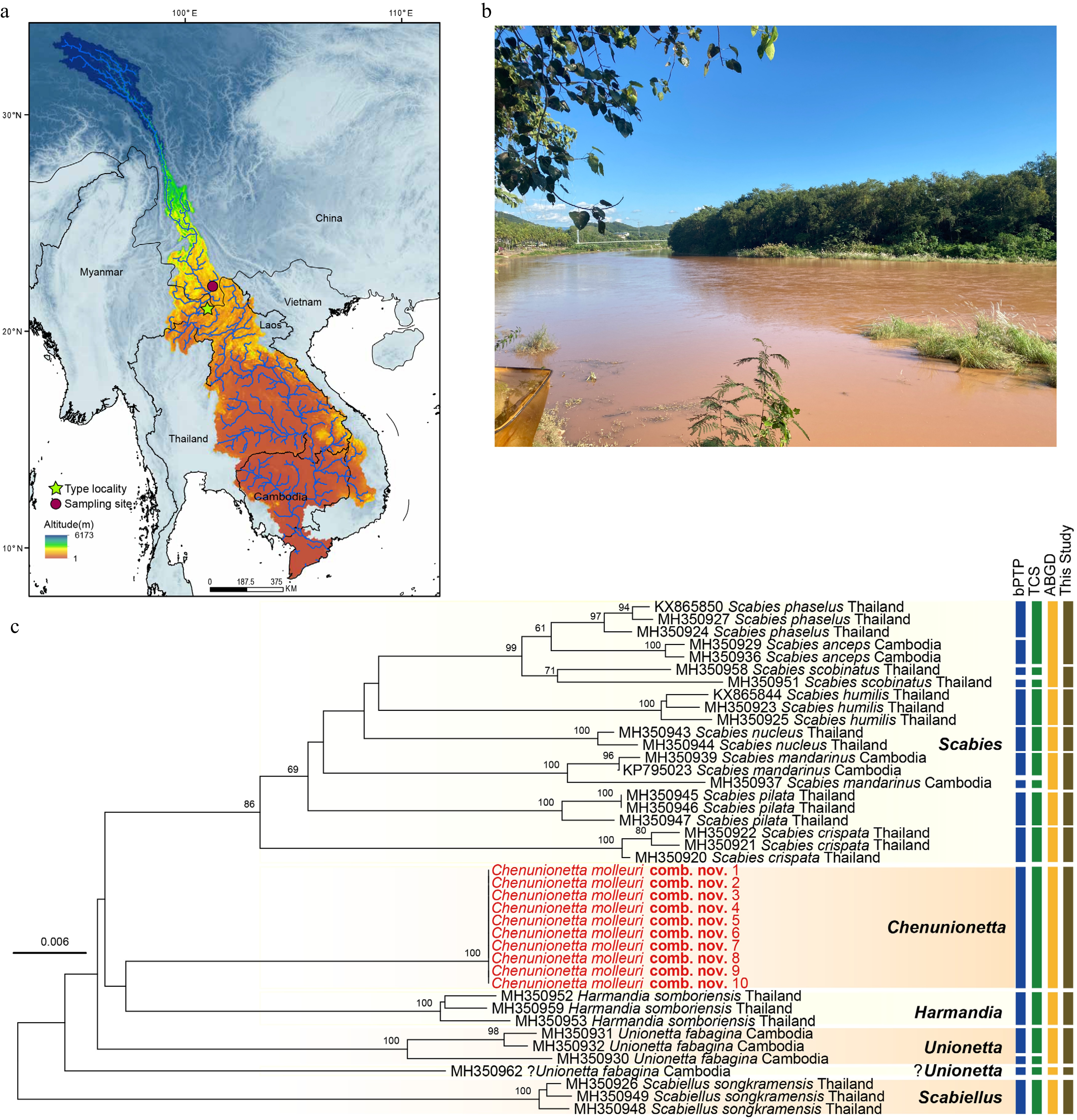
Figure 1. 

Sampling locality and species delimitation of Chenunionetta molleuri comb. nov. (a), (b) Map and general view of the sampling locality. The map was generated using ArcGIS (v10.2, Esri, Redlands, CA, USA). (c) Neighbor-joining tree of 224 COI sequences (Supplementary Fig. S1), based on Kimura 2-parameter model with 1,000 bootstrap replicates. Bootstrap support values ≥ 50% are shown at the nodes. Tip labels of Chenunionetta lineage are highlighted in red. Results from three delimitation analyses are shown; colored bars indicate inferred groupings and allow visual comparison of congruence among methods.

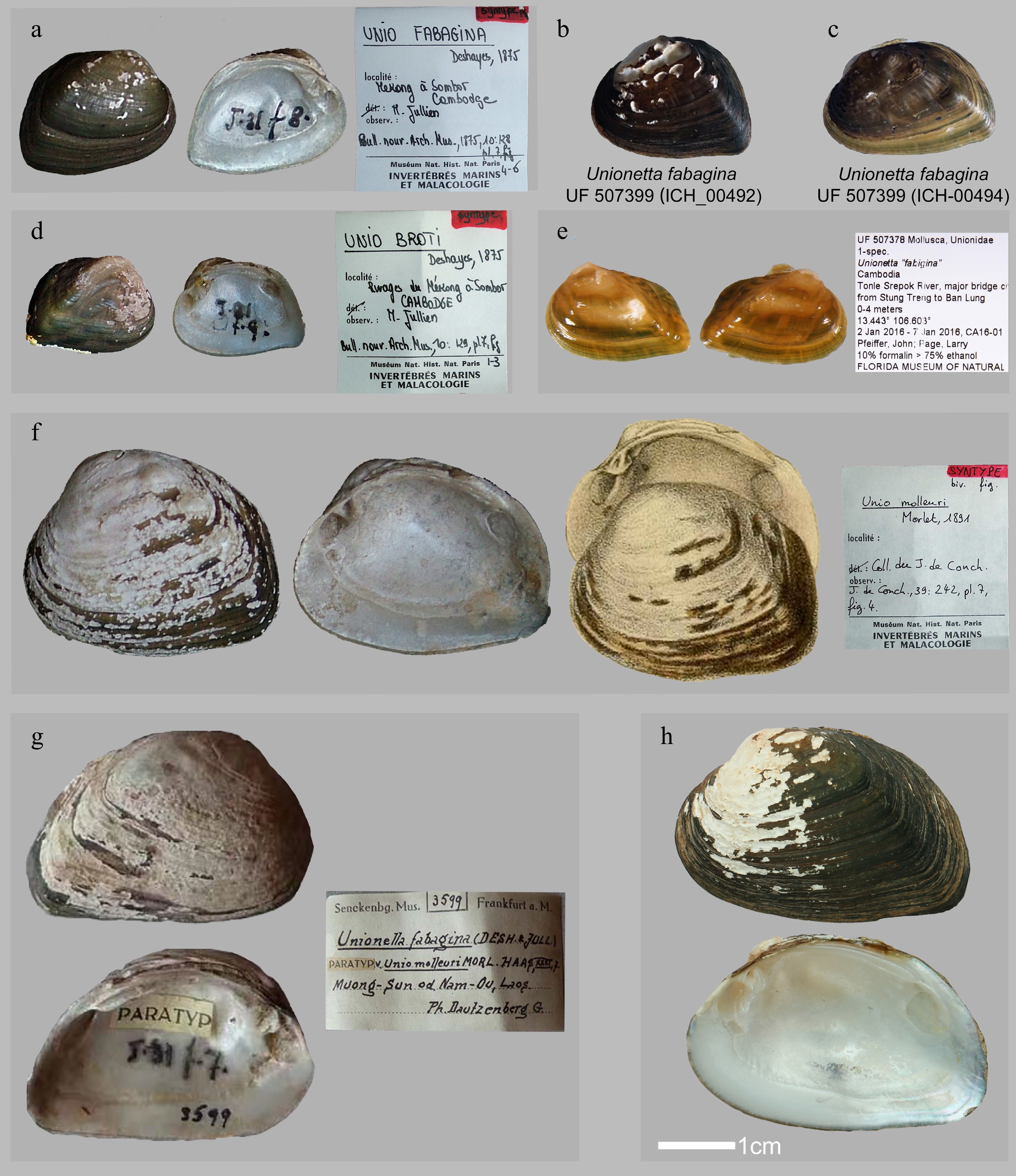
Figure 2. 

Shells of Unionetta fabagina species complex. (a) Unionetta fabagina (Unio fabagina Deshayes, 1876, syntype MNHN-IM-2000-1694). (b), (c) Sequenced specimens of Unionetta fabagina in Pfeiffer et al. (2018)^[11]. (d) Unionetta fabagina (Unio broti Deshayes, 1876, syntype MNHN-IM-2000-1652). (e) ?Unionetta fabagina in Pfeiffer et al. (2018)^[11]. (f)–(h) Unio molleuri Morlet, 1891 (Syntype MNHN-IM-2000-1751, paratype SMF 3599, and NCUMB 21_NCU_XPWU_UF10, respectively). Scale bar in (h) = 1 cm and applies only to panel (h); remaining panels are scaled proportionally to reflect approximate size differences among specimens.

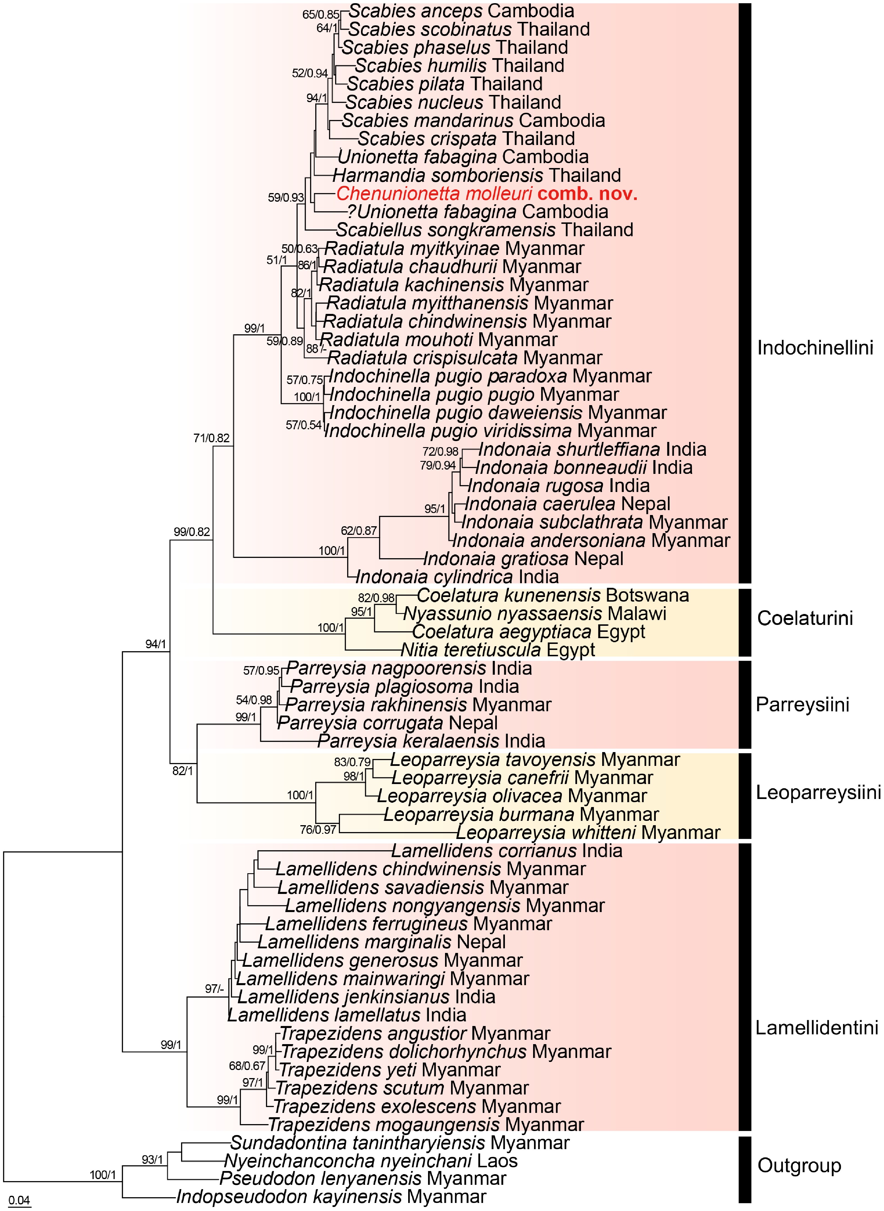
Figure 3. 

Maximum likelihood phylogenetic tree based on the concatenated three-gene dataset (COI + 16S + 28S; 1,866 bp). Tip label of Chenunionetta lineage is highlighted in red. Nodal support values are shown as ML bootstrap/BI posterior probability, with dashes indicating nodes that conflict between the two inference methods. Bootstrap support values ≥ 50% or posterior probability ≥ 0.5 are shown at the nodes.

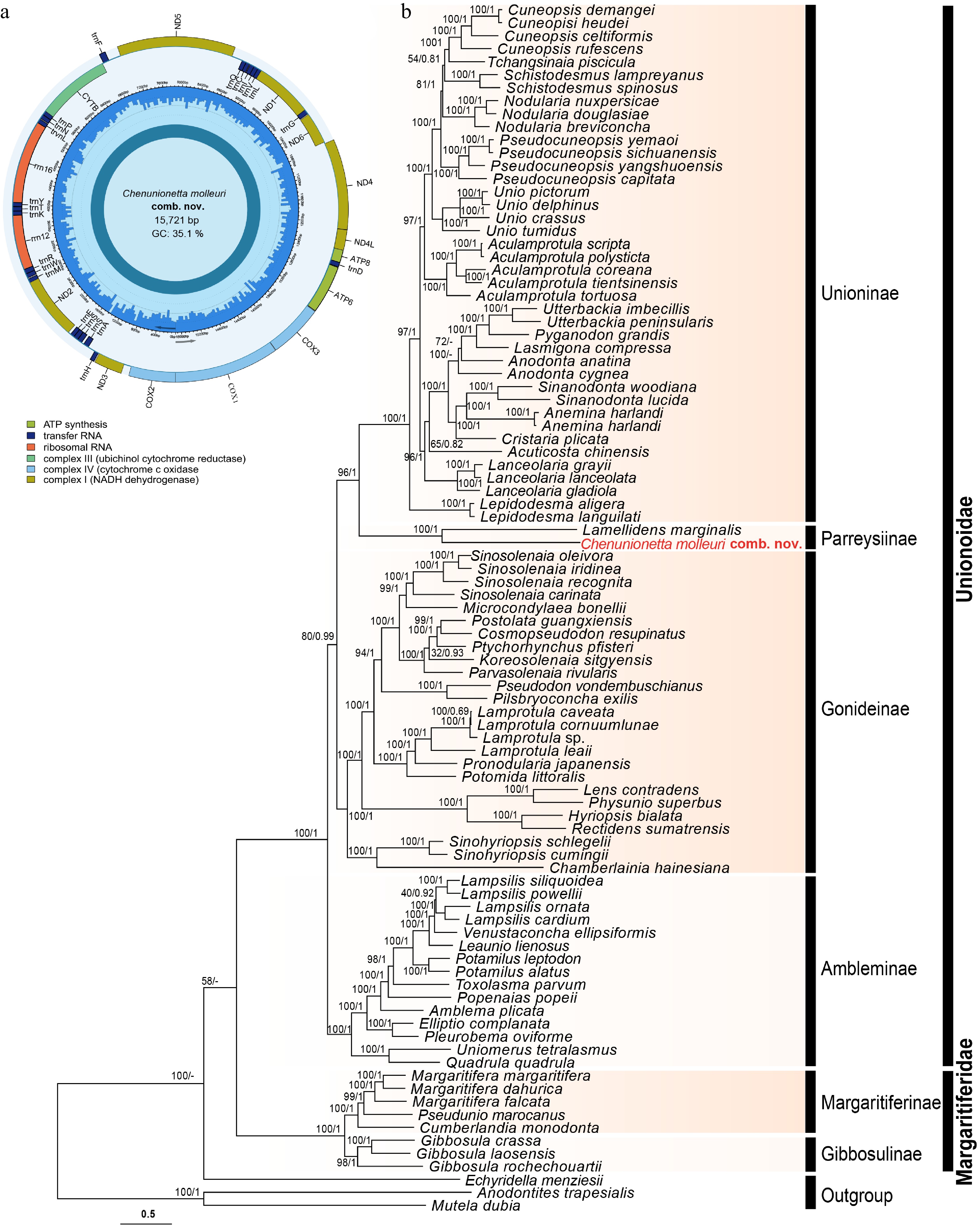
Figure 4. 

Analysis based on mitochondrial data. (a) Gene map of the F-type mitochondrial genome of Chenunionetta molleuri comb. nov. (b) Maximum likelihood phylogeny based on the F-type complete mitochondrial genome dataset (12 PCGs and 2 rRNAs). Tip label of Chenunionetta lineage is highlighted in red. Nodal support values (bootstrap from RAxML/posterior probability from MrBayes) are annotated on branches, with dashes indicating nodes that conflict between the two inference methods.

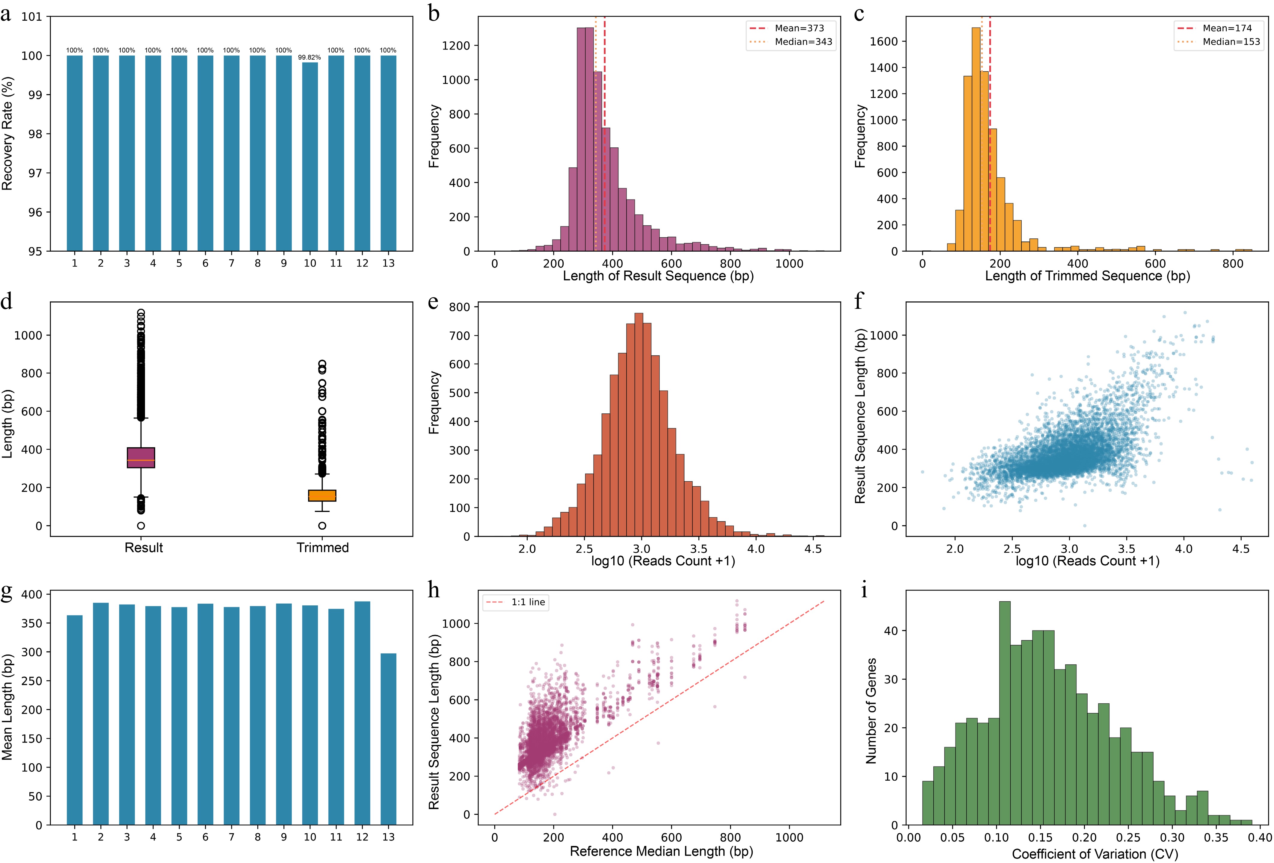
Figure 5. 

Summary statistics of in silico AHE gene capture across 13 Unionidae samples. (a) Gene recovery rate for each sample. (b) Frequency distribution of result sequence lengths with mean (red dashed line) and median (orange dotted line) indicated. (c) Frequency distribution of trimmed sequence lengths with mean and median indicated. (d) Length comparison between result and trimmed sequences. (e) Distribution of read counts on a log₁₀ scale. (f) Scatter plot showing the relationship between result sequence length and read depth (log₁₀ scale). (g) Mean result sequence length per sample. (h) Comparison of result sequence length with reference median length; the dashed line indicates the 1:1 relationship. (i) Distribution of the coefficient of variation (CV) of result sequence length across the 569 AHE loci.

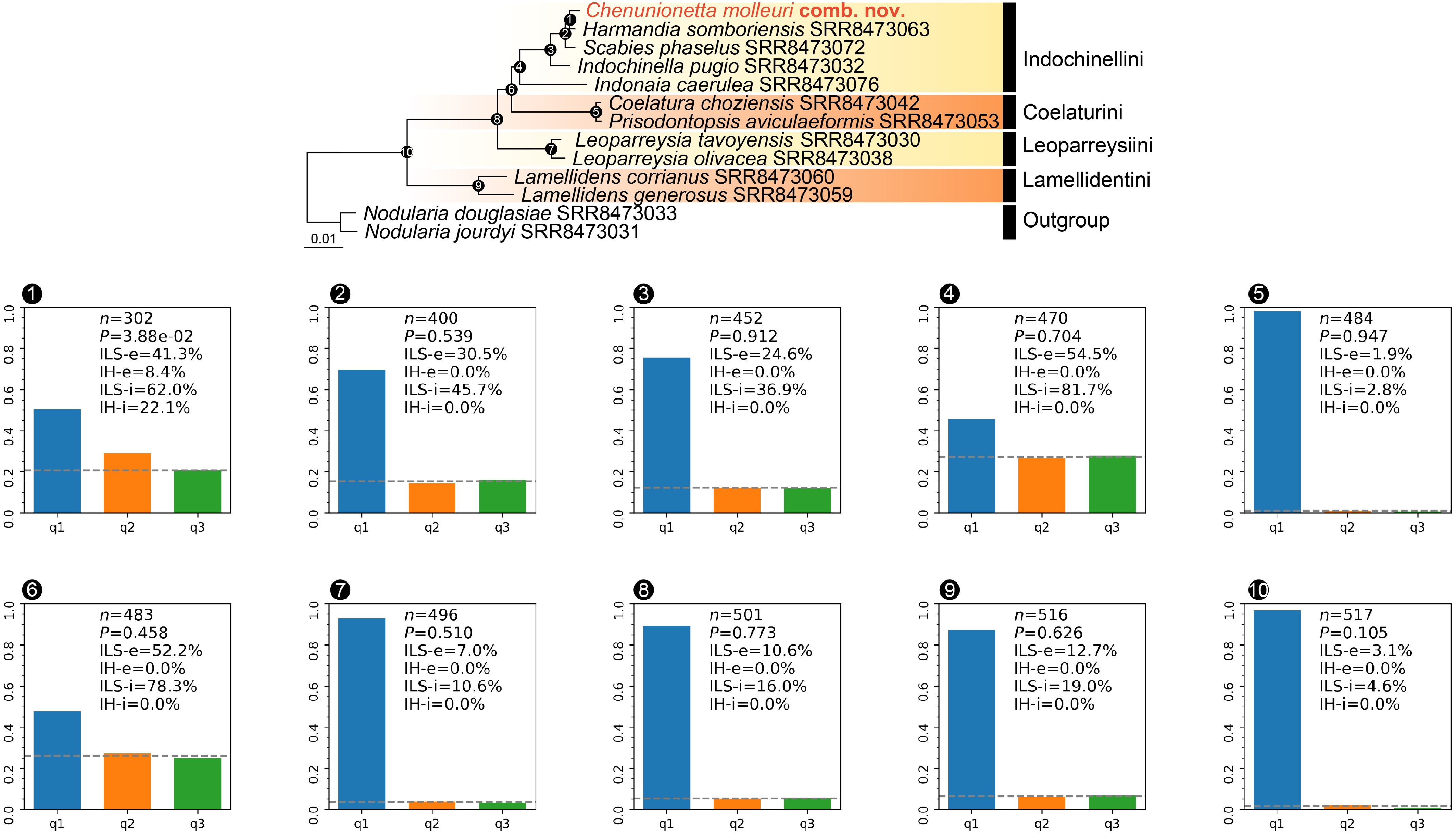
Figure 6. 

ASTRAL-III species tree inferred from 569 in silico-captured AHE nuclear loci. Branch support values (ASTRAL-III local posterior probabilities, IQ-TREE ultrafast bootstrap, and FastTree local support values) were uniformly maximal (100%) at all nodes and are therefore omitted for clarity. Insets display the quartet-based discordance analyses at the corresponding numbered nodes (1–10). Tip label of Chenunionetta is highlighted in red.