-
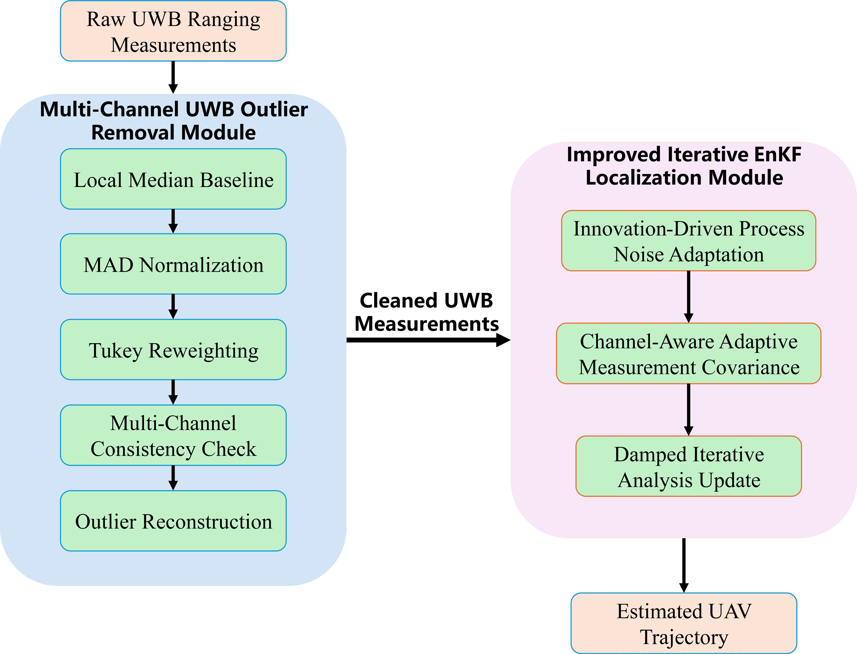
Figure 1.
Structure of the proposed robust indoor UWB localization framework.
-
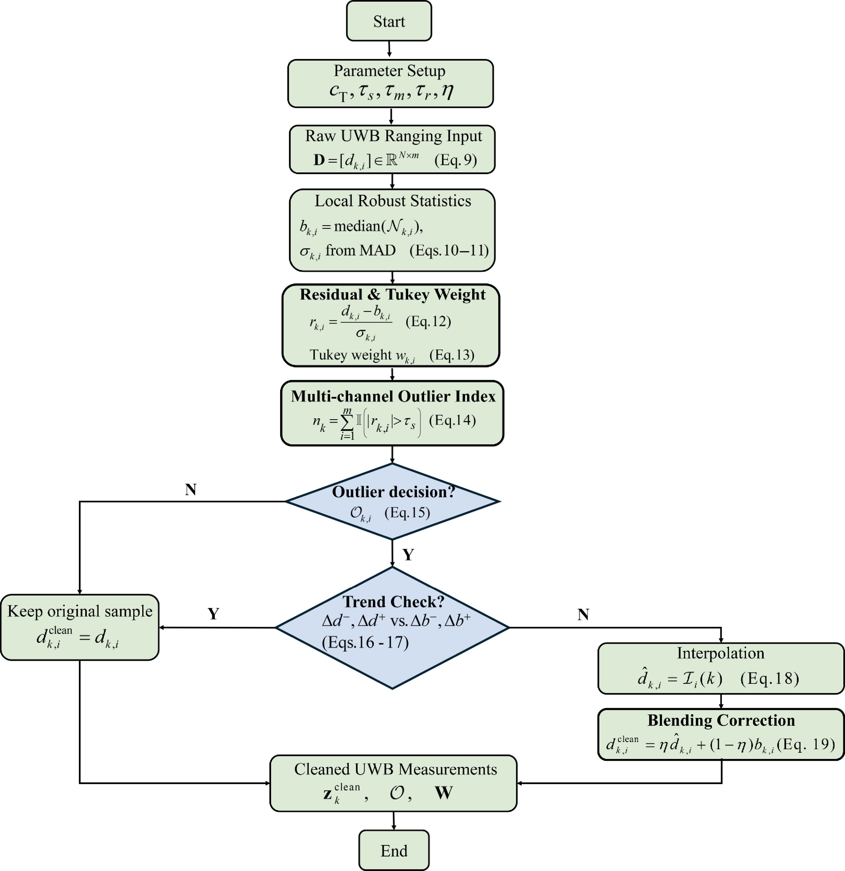
Figure 2.
Workflow of the proposed UWB outlier removal algorithm.
-
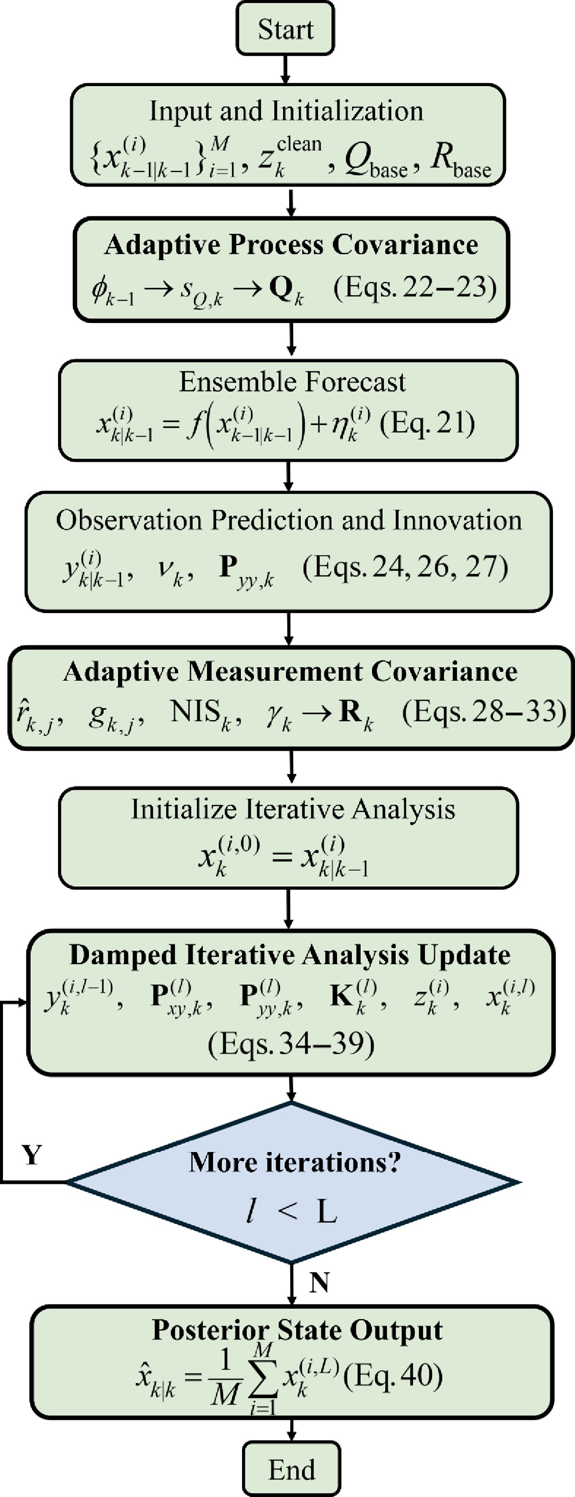
Figure 3.
Workflow of the proposed improved iterative ensemble Kalman filter backend.
-
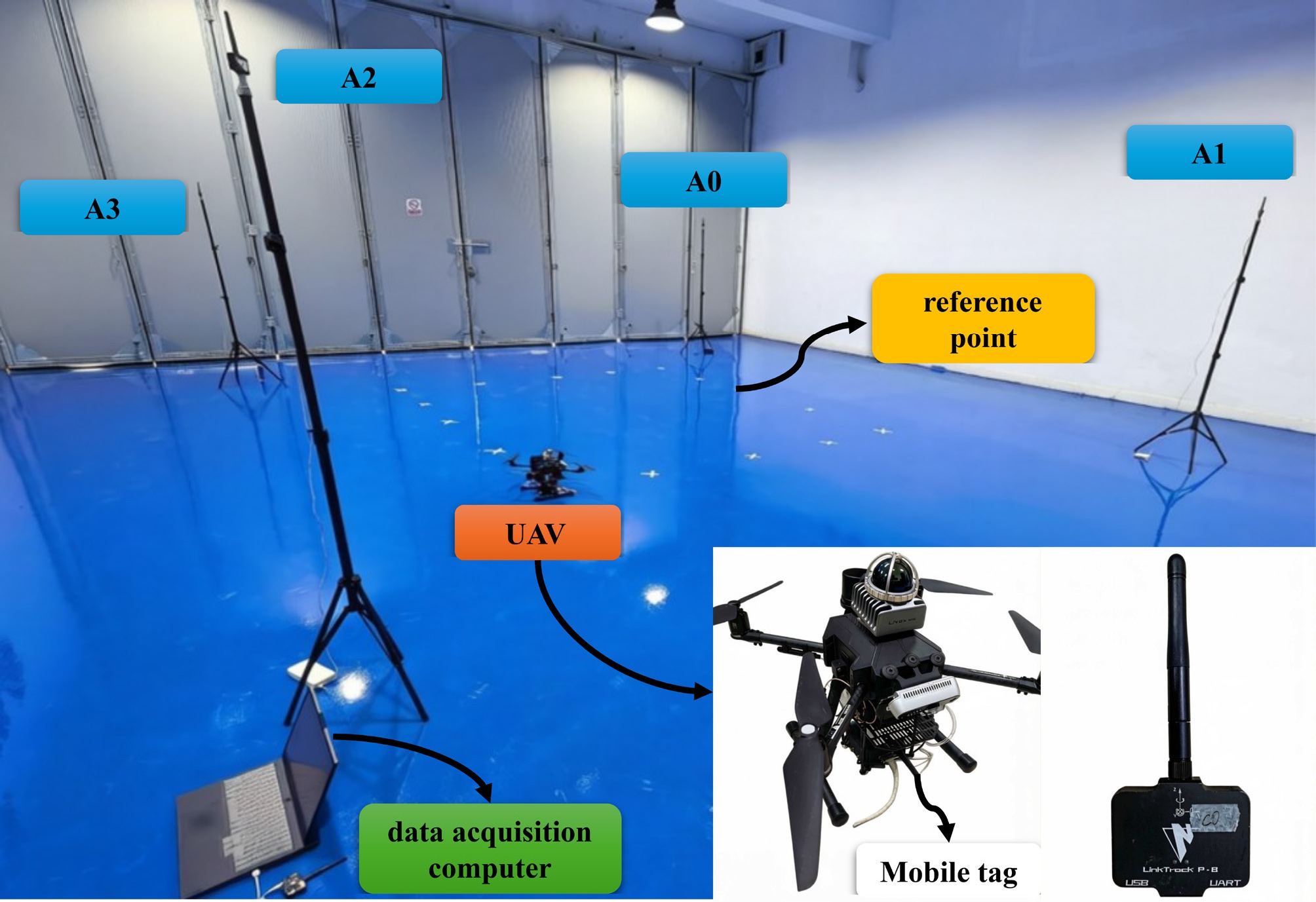
Figure 4.
Experimental setup of the indoor UWB localization test, including four fixed anchors, the UAV-mounted mobile tag, reference points, and the data acquisition computer.
-
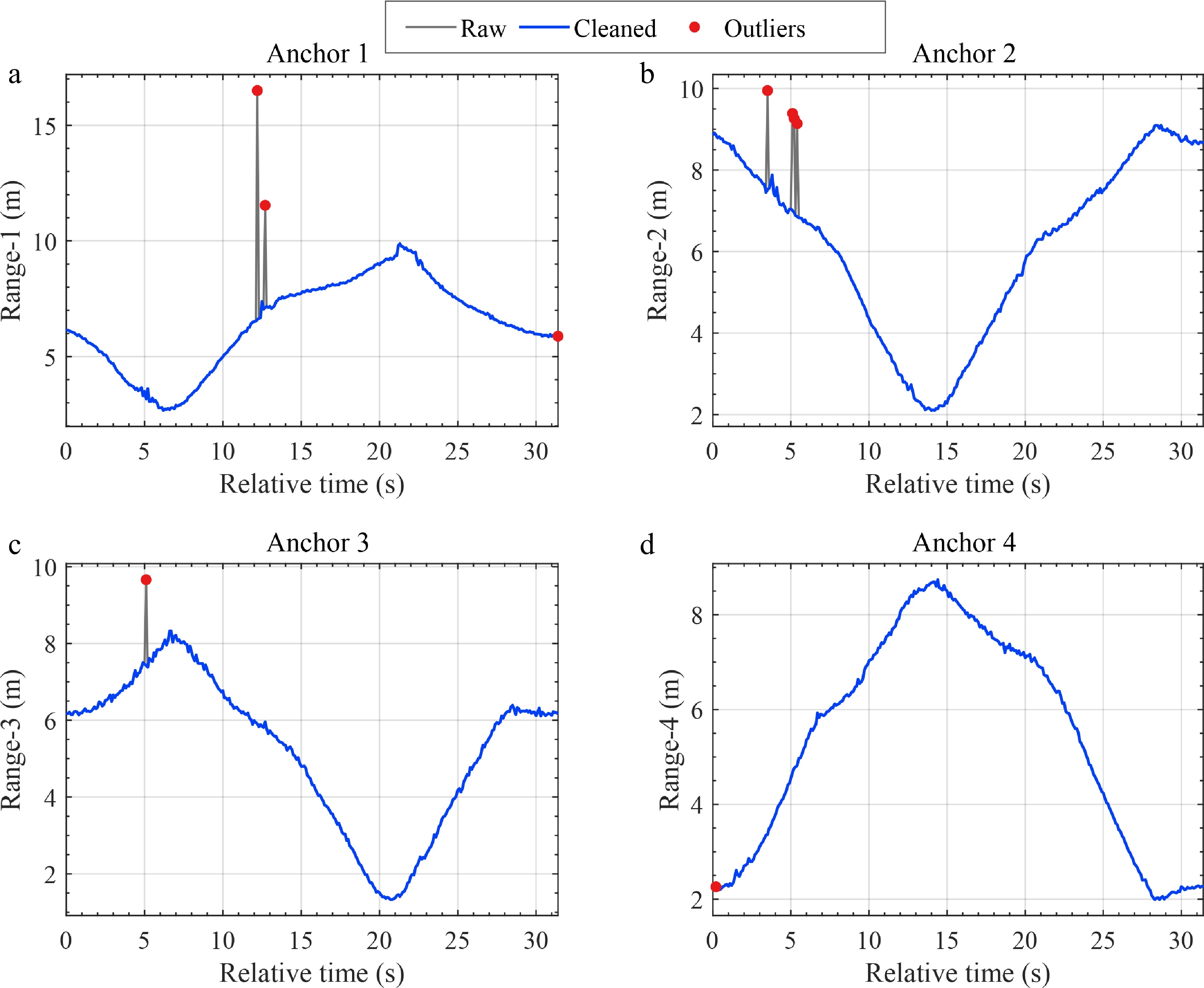
Figure 5.
UWB range measurements before and after multi-channel outlier removal in one representative experimental run.
-
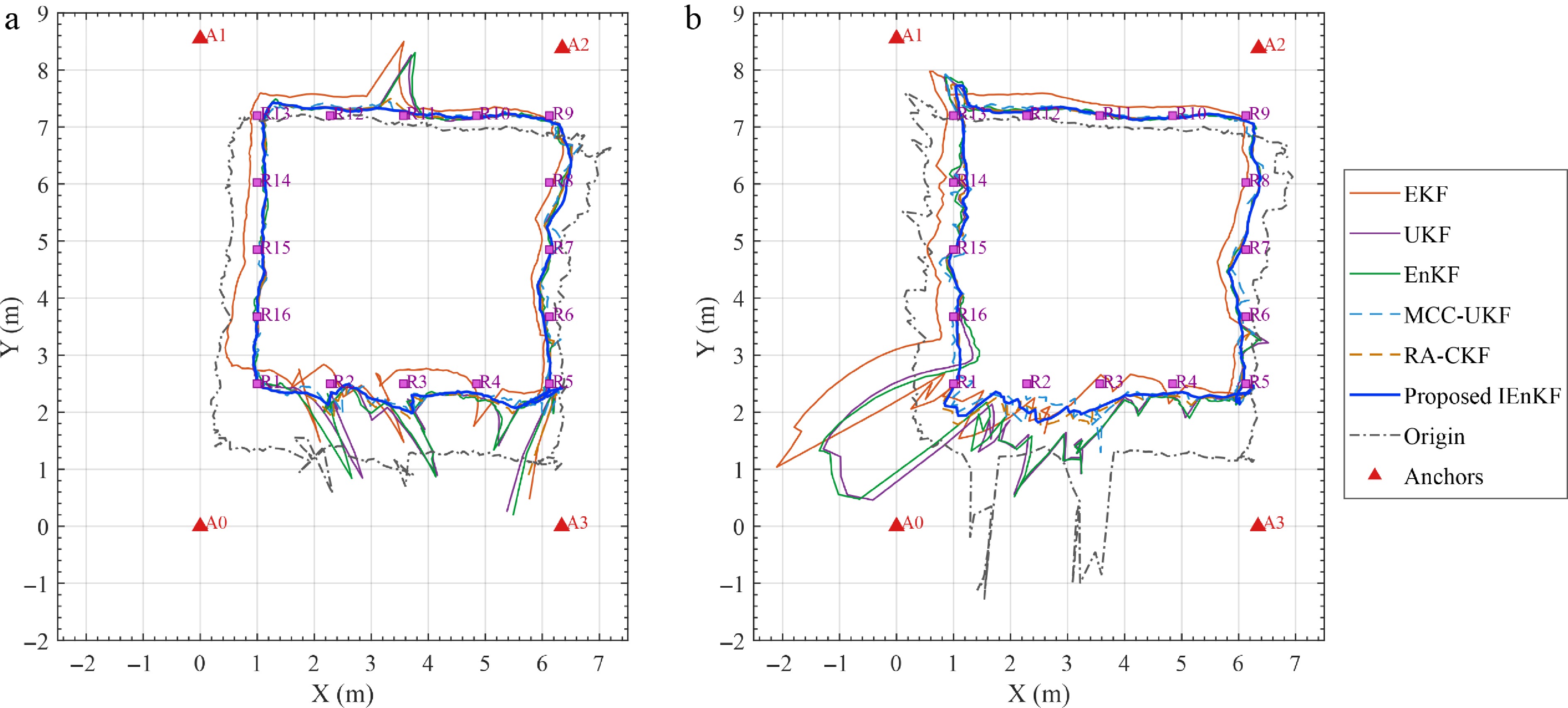
Figure 6.
Two-dimensional trajectory comparison of different localization methods in two representative experimental runs. (a) Representative run 1. (b) Representative run 2.
-
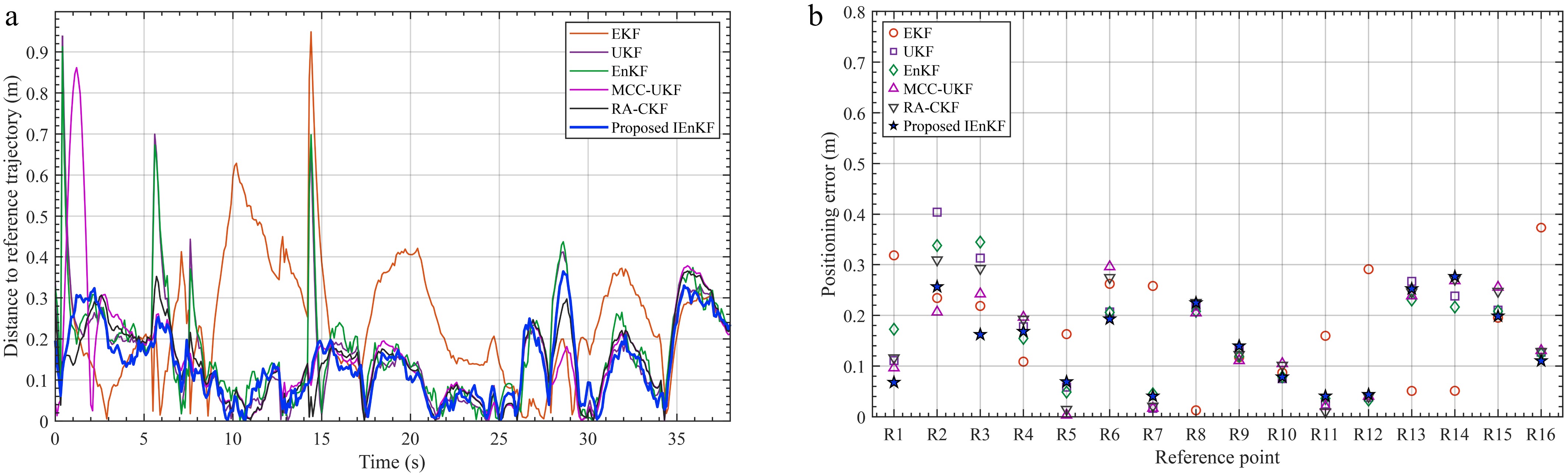
Figure 7.
Trajectory-to-reference-path deviation and reference-point positioning error comparison of different filtering methods in one representative experimental run. (a) Trajectory-to-reference-path deviation. (b) Reference-point positioning error.
-
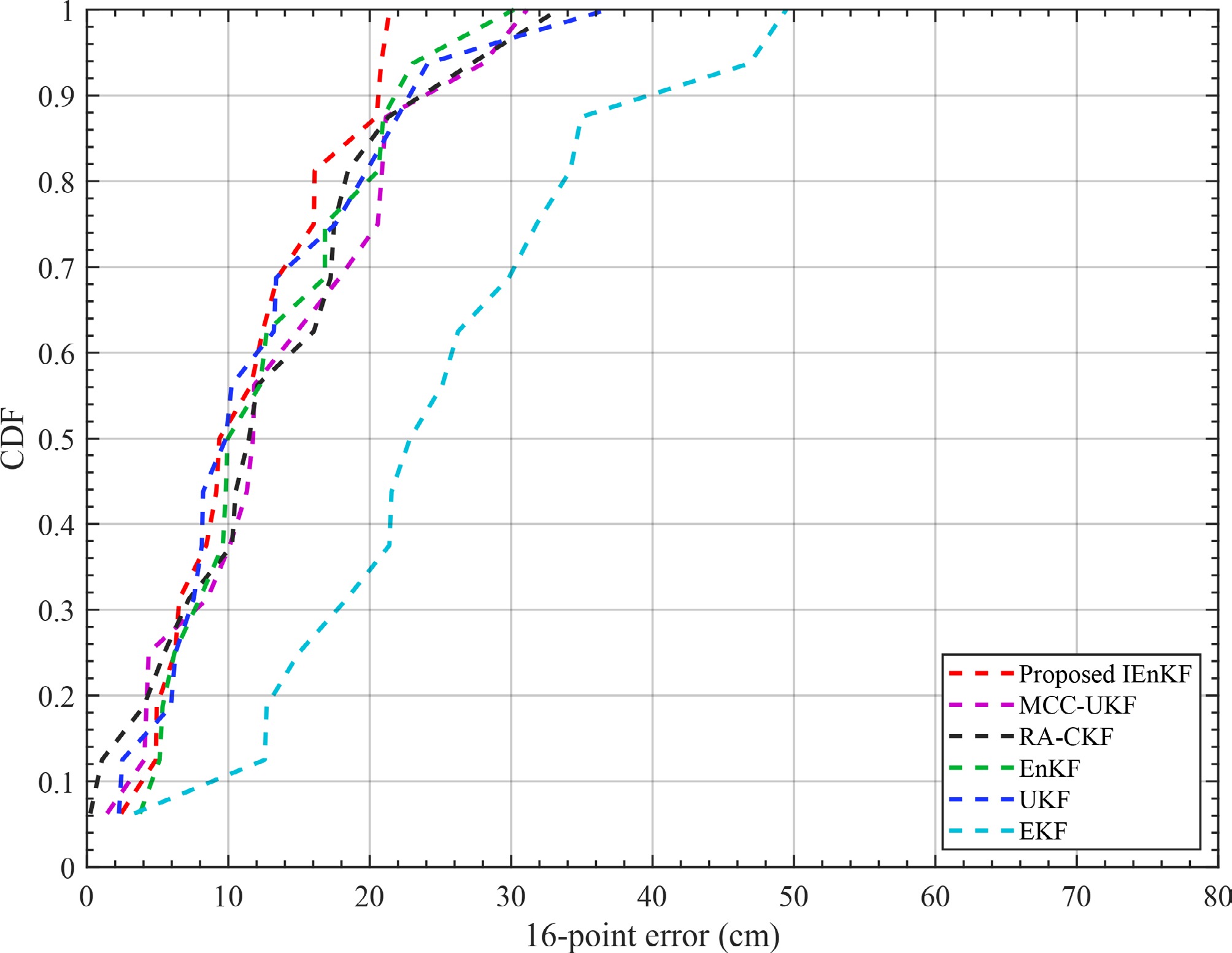
Figure 8.
CDF curves of reference-point positioning errors for different filtering methods in one representative experimental run.
-
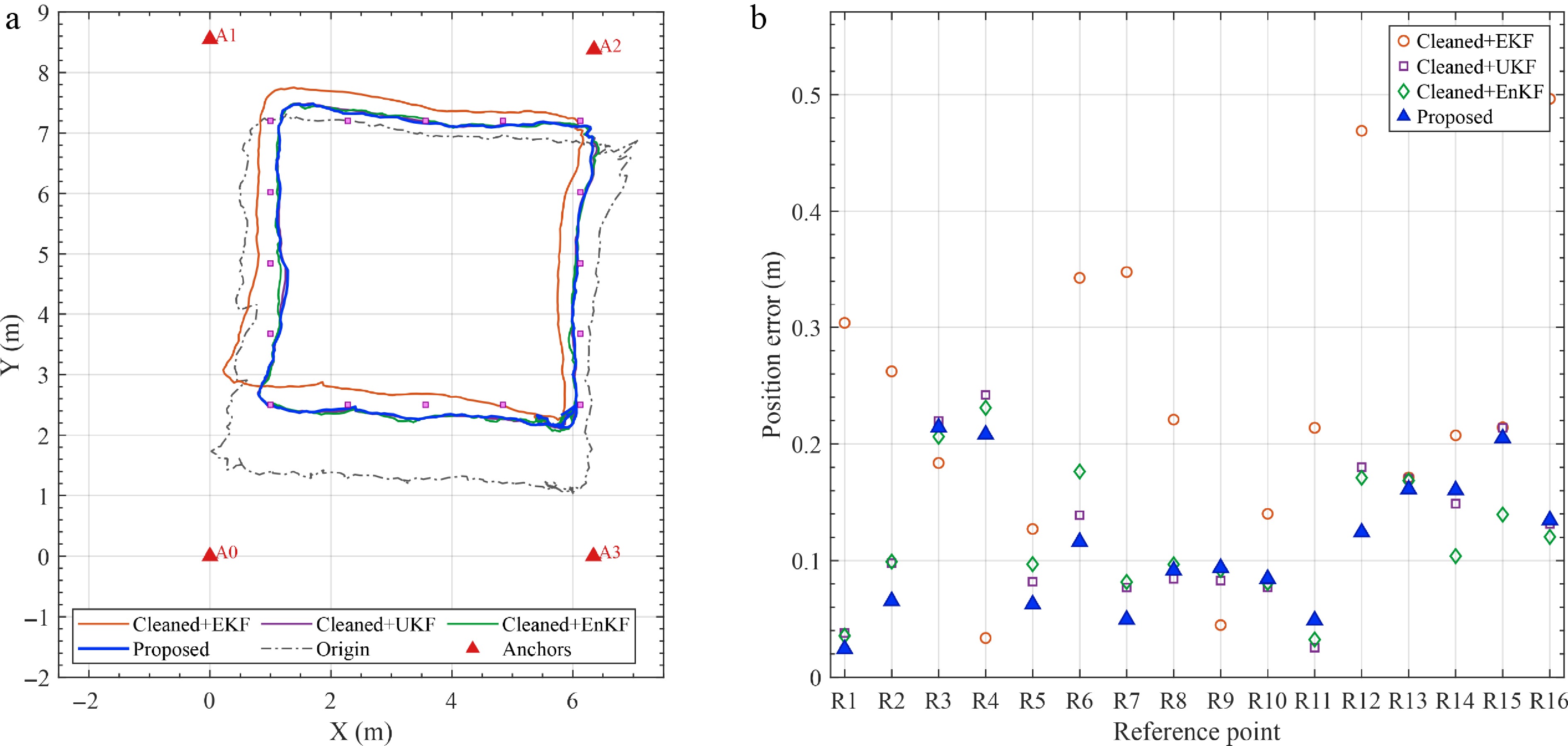
Figure 9.
Backend filter comparison under the same cleaned UWB measurements in one representative experimental run. (a) Two-dimensional trajectory comparison. (b) Reference-point positioning errors.
-
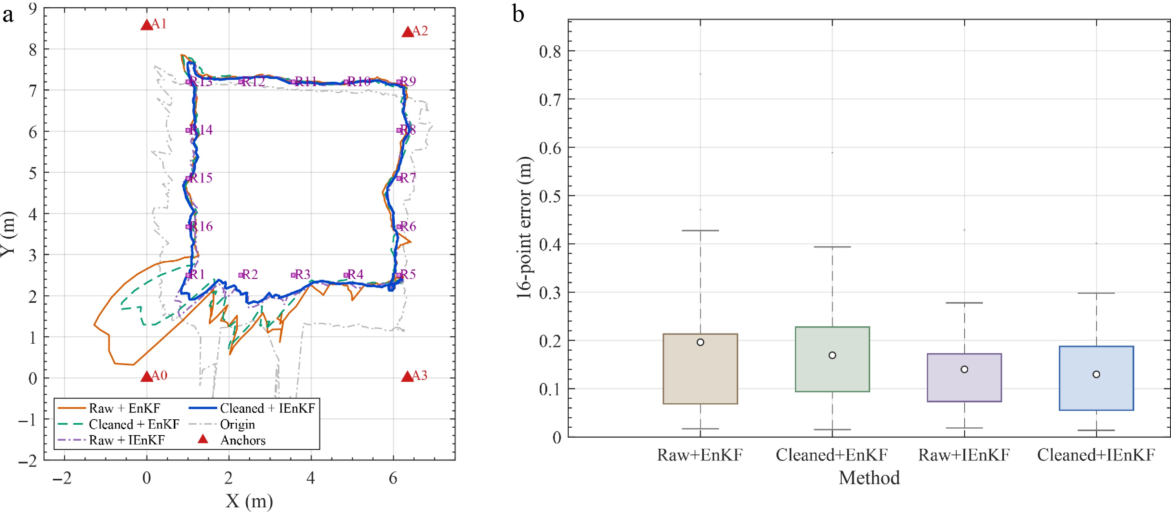
Figure 10.
Ablation comparison of different front-end and back-end configurations in one representative experimental run. (a) Two-dimensional trajectory comparison. (b) Reference-point positioning error distribution.
-
Input: Previous posterior ensemble $ \{{\boldsymbol{x}}_{k-1|k-1}^{(i)}\}_{i=1}^{M} $ $ {\boldsymbol{z}}_{k}^{{\rm{clean}}} $ $ {\boldsymbol{f}}(\cdot) $ $ {\boldsymbol{h}}(\cdot) $ Output: Posterior state estimate $ \hat{{\boldsymbol{x}}}_{k|k} $ 1: Adapt $ {\boldsymbol{Q}}_k $ 2: for $ i = 1 $ $ M $ 3: Draw process noise $ {\boldsymbol{\eta}}_{k}^{(i)} \sim {\cal{N}}({\boldsymbol{0}}, {\boldsymbol{Q}}_k) $ 4: Predict ensemble member: ${\boldsymbol{x}}_{k|k-1}^{(i)} = {\boldsymbol{f}} \left({\boldsymbol{x}}_{k-1|k-1}^{(i)}\right) + {\boldsymbol{\eta}}_{k}^{(i)} $ 5: end for 6: Compute forecast ensemble mean $ \bar{{\boldsymbol{x}}}_{k|k-1} $ 7: Compute predicted measurements $ {\boldsymbol{y}}_{k|k-1}^{(i)} = {\boldsymbol{h}}({\boldsymbol{x}}_{k|k-1}^{(i)}) $ 8: Compute innovation and residual statistics using $ {\boldsymbol{z}}_{k}^{{\rm{clean}}}-\bar{{\boldsymbol{y}}}_{k|k-1} $ 9: Construct channel-aware $ {\boldsymbol{R}}_k $ 10: Initialize the iterative analysis with $ {\boldsymbol{x}}_{k}^{(i,0)} = {\boldsymbol{x}}_{k|k-1}^{(i)} $ 11: for $ \ell = 1 $ $ L $ 12: Propagate the current ensemble through the nonlinear measurement function 13: Compute the sample cross-covariance and innovation covariance 14: Compute the Kalman gain $ {\boldsymbol{K}}_{k}^{(\ell)} $ 15: Perform the damped ensemble update with damping factor $ \mu_{\ell} $ 16: end for 17: Compute the posterior state estimate: $\hat{{\boldsymbol{x}}}_{k|k} = \dfrac{1}{M}\sum\limits_{i=1}^{M}{\boldsymbol{x}}_{k}^{(i,L)} $ Table 1.
Improved IEnKF for indoor UWB localization
-
Item Value UWB device Nooploop LinkTrack UWB modules Number of UWB anchors 4 Anchor coordinates $ {\rm{A0:}}\;(0,0)\; {\rm{m}} \quad {\rm{~A}} 1:(0,8.55)\; {\rm{m}}$ ${\rm{A2:}}\;(6.35,8.38)\; {\rm{m}} \quad {\rm{~A}} 3:(6.34,0) \;{\rm{m}} $ Sampling rate 10 Hz (0.1 s sampling interval) Table 1.
Main experimental setup of the indoor UWB localization test.
-
Channel Raw
STD (m)Cleaned
STD (m)Detected
outlier ratio (%)Detected
outlier countAnchor 1 0.1708 0.0594 0.68 10 Anchor 2 0.3682 0.0942 1.84 27 Anchor 3 0.4718 0.2308 2.23 33 Anchor 4 0.1353 0.0669 1.20 18 Table 2.
UWB ranging residual statistics before and after front-end preprocessing over four experimental runs.
-
Method Path RMSE (m) Path MAE (m) Ref. RMSE (m) Ref. MAE (m) EKF 0.3549 0.2642 0.2312 0.2028 UKF 0.3323 0.2182 0.1901 0.1511 EnKF 0.3463 0.2295 0.1860 0.1492 MCC-UKF 0.2404 0.1847 0.1588 0.1336 RA-CKF 0.2215 0.1822 0.1762 0.1439 Proposed IEnKF 0.1888 0.1586 0.1451 0.1243 Table 3.
Overall reference-point/path-deviation performance comparison of different methods over four experimental runs.
-
Method RMSE (m) MAE (m) Cleaned + EKF 0.2359 0.2036 Cleaned + UKF 0.1765 0.1439 Cleaned + EnKF 0.1713 0.1391 Proposed IEnKF 0.1451 0.1243 Table 4.
Reference-point localization errors of different backend filters under the same cleaned UWB measurements over four experimental runs.
-
Method RMSE (m) MAE (m) Raw + EnKF 0.1860 0.1492 Cleaned + EnKF 0.1713 0.1391 Raw + IEnKF 0.1708 0.1442 Cleaned + IEnKF 0.1451 0.1243 Table 5.
Ablation results of different front-end and backend configurations over four experimental runs.
-
Method Adap. Q Ch.-aware R Damped RMSE MAE MAX EnKF × × × 0.1713 0.1391 0.3770 IEnKF × × √ 0.1625 0.1316 0.3570 Proposed w/o adaptive Q × √ √ 0.1502 0.1260 0.2862 Proposed w/o Ch.-aware R √ × √ 0.1682 0.1355 0.3792 Proposed w/o damping √ √ × 0.1503 0.1269 0.2905 Full proposed √ √ √ 0.1451 0.1243 0.2820 Table 6.
Component-level ablation results of the proposed backend mechanisms over four experimental runs.
-
(a) Proposed IEnKF under different anchor configurations Anchor configuration RMSE (m) MAE (m) MAX (m) A0-A1-A2-A3 0.1451 0.1243 0.2820 A1-A2-A3 0.1679 0.1379 0.4002 A0-A2-A3 0.2309 0.1714 0.6389 A0-A1-A3 0.2082 0.1705 0.4525 A0-A1-A2 0.1594 0.1320 0.3355 (b) RMSE under synthetic NLOS and dynamic occlusion stress tests Stress case EKF UKF EnKF MCC-UKF RA-CKF Proposed IEnKF Original 0.2312 0.1901 0.1860 0.1588 0.1762 0.1451 5% NLOS bias 0.2367 0.2041 0.2074 0.1694 0.1937 0.1589 10% NLOS bias 0.2294 0.2071 0.2089 0.1747 0.1985 0.1575 15% NLOS bias 0.2325 0.2095 0.2132 0.1842 0.2074 0.1687 Dynamic occlusion 0.2301 0.2116 0.2157 0.1737 0.2009 0.1620 Table 7.
Controlled post-processing robustness analysis under anchor-channel removal and synthetic ranging disturbances.
-
Parameter Tested values Recommended value Avg. best RMSE (m) Avg. RMSE range (m) Sensitivity Tukey cutoff 2.5/3.0/3.5/4.0 2.5 0.1457 0.0022 Low Window size 5/7/9/11 7 0.1446 0.0030 Low Ensemble size 30/50/80/100/120 100 0.1415 0.0098 Low Iteration number 1/2/3/4/5 3 0.1407 0.0201 Medium Q scaling bound 2/3/4/5 2 0.1460 0.0000 Low R clipping bound 1.5/2.5/3.5/4.5 1.5 0.1424 0.0118 Low Table 8.
Parameter sensitivity results of the proposed localization framework.
Figures
(10)
Tables
(9)