-
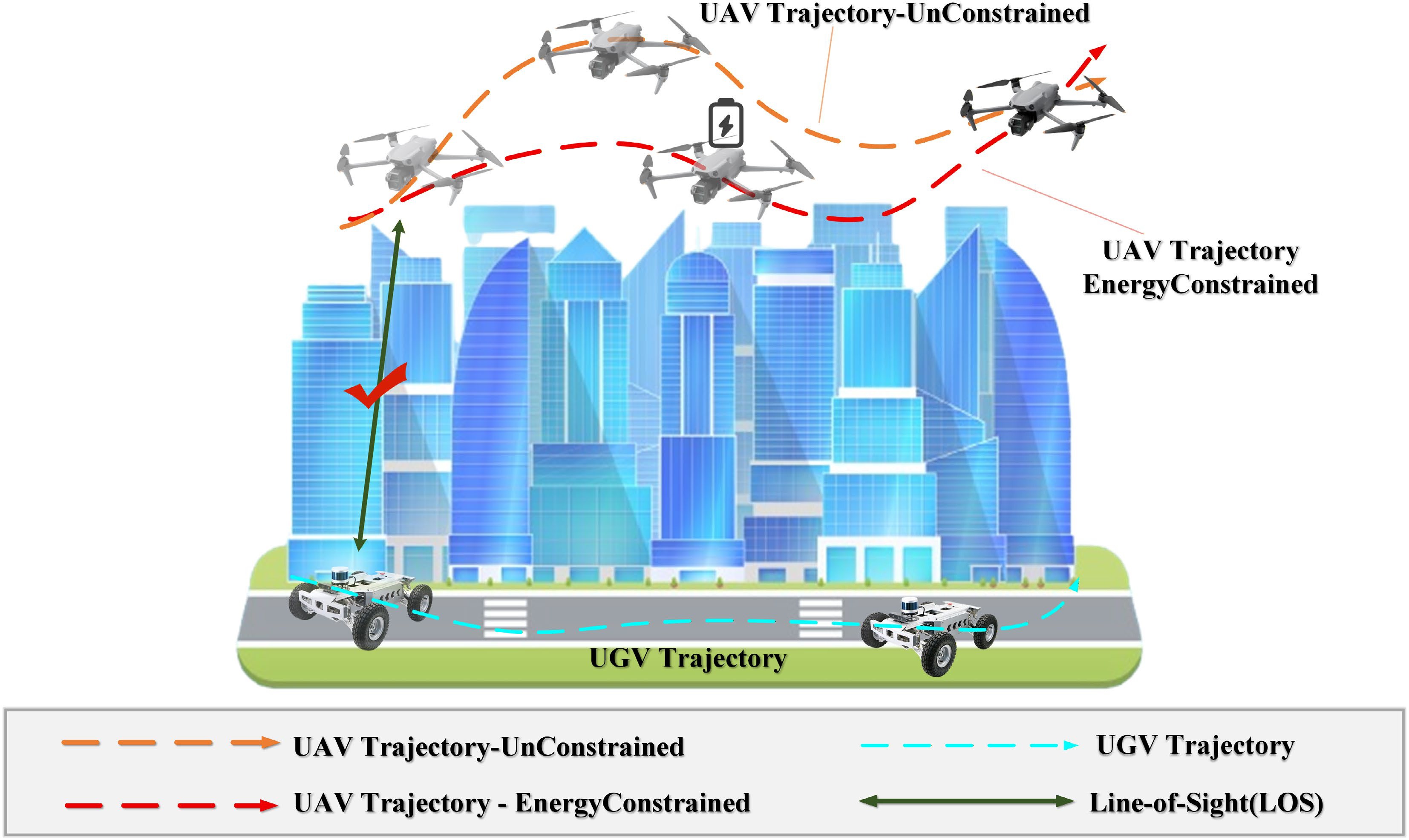
Figure 1.
An illustration of a heterogeneous UAV and UGV systems operating in a cluttered environment. The UAV performs forward reconnaissance while maintaining LOS with the UGV and planning an energy-efficient trajectory toward the goal, accounting for LOS occlusions caused by obstacles.
-
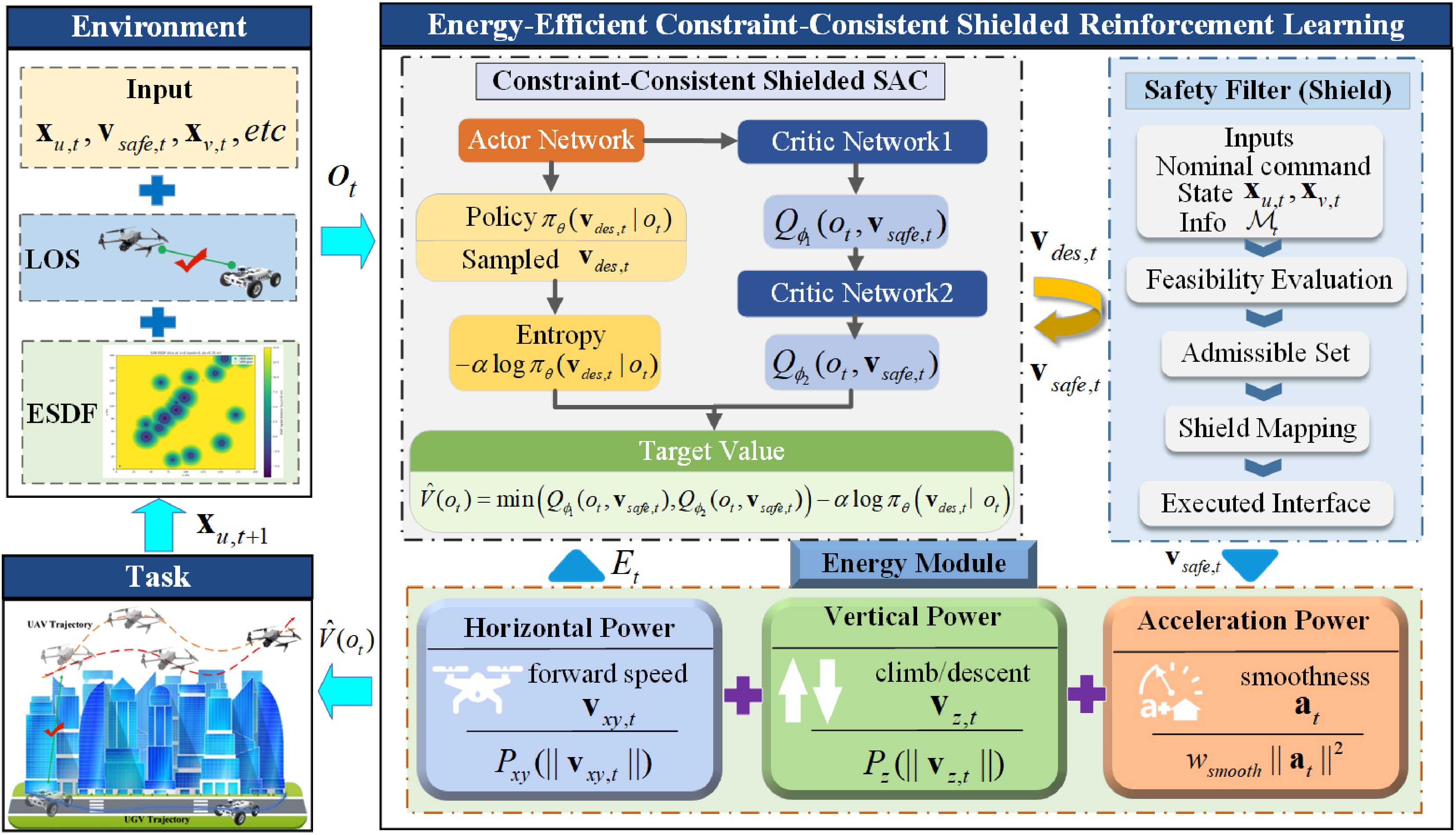
Figure 2.
Framework of the proposed method.
-
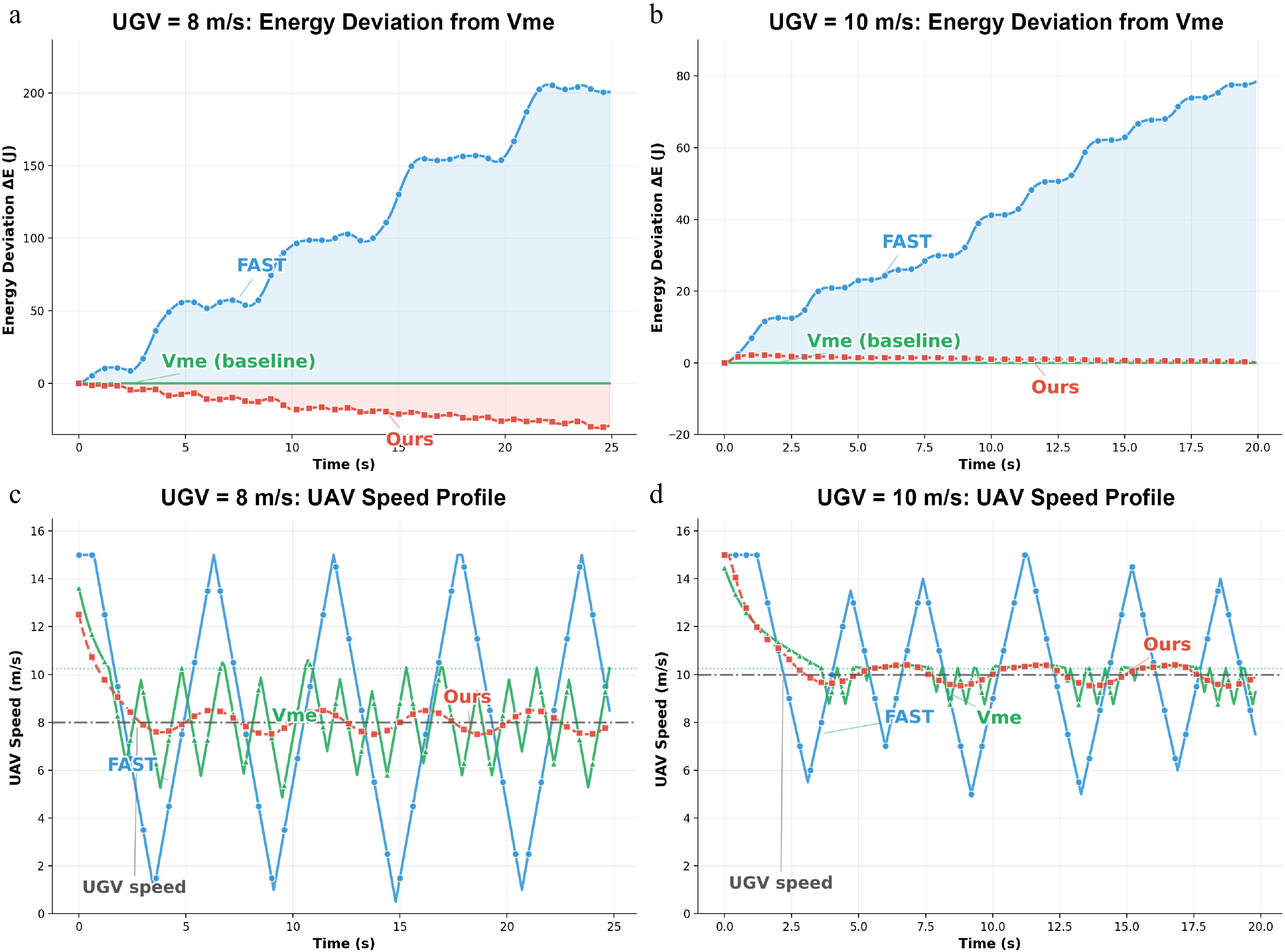
Figure 3.
Constraint-inactive comparison relative to Vme. (a), (b) Cumulative energy deviation
$ \Delta E(t) $ $ v_g\in\{8,10\}\,\mathrm{m/s} $ -
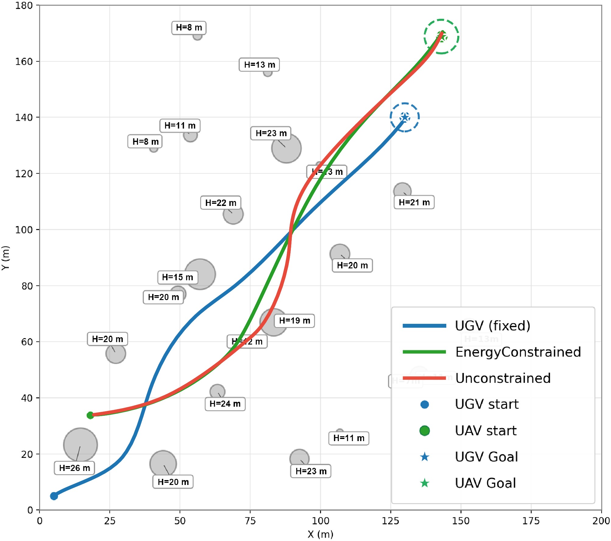
Figure 4.
Scenario 1 (initial NLOS): planar trajectories of the UGV and UAV.
-
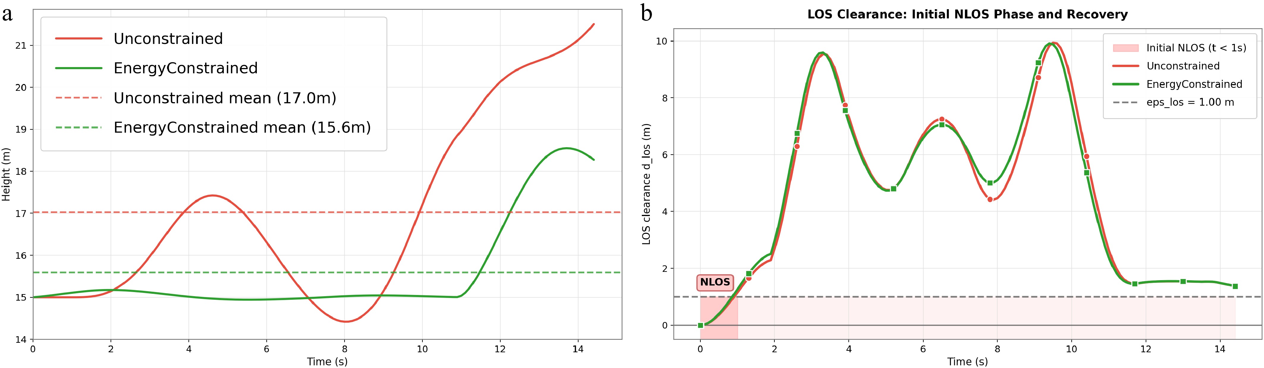
Figure 5.
Scenario 1 (initial NLOS): altitude evolution and LOS clearance for Unconstrained and EnergyConstrained. (a) UAV height profiles. (b) LOS clearance/margin metric.
-
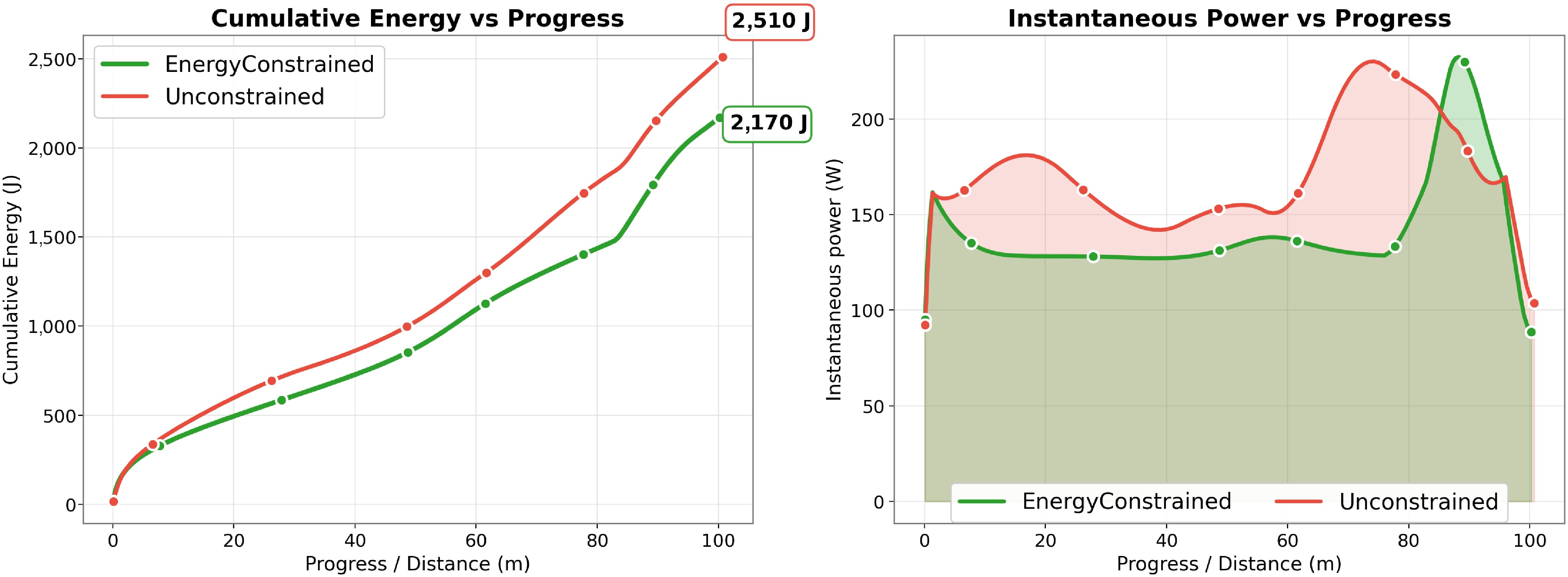
Figure 6.
Scenario 1 (initial NLOS): cumulative propulsion energy aligned by progress and instantaneous power computed from executed velocities using Eq. (40).
-
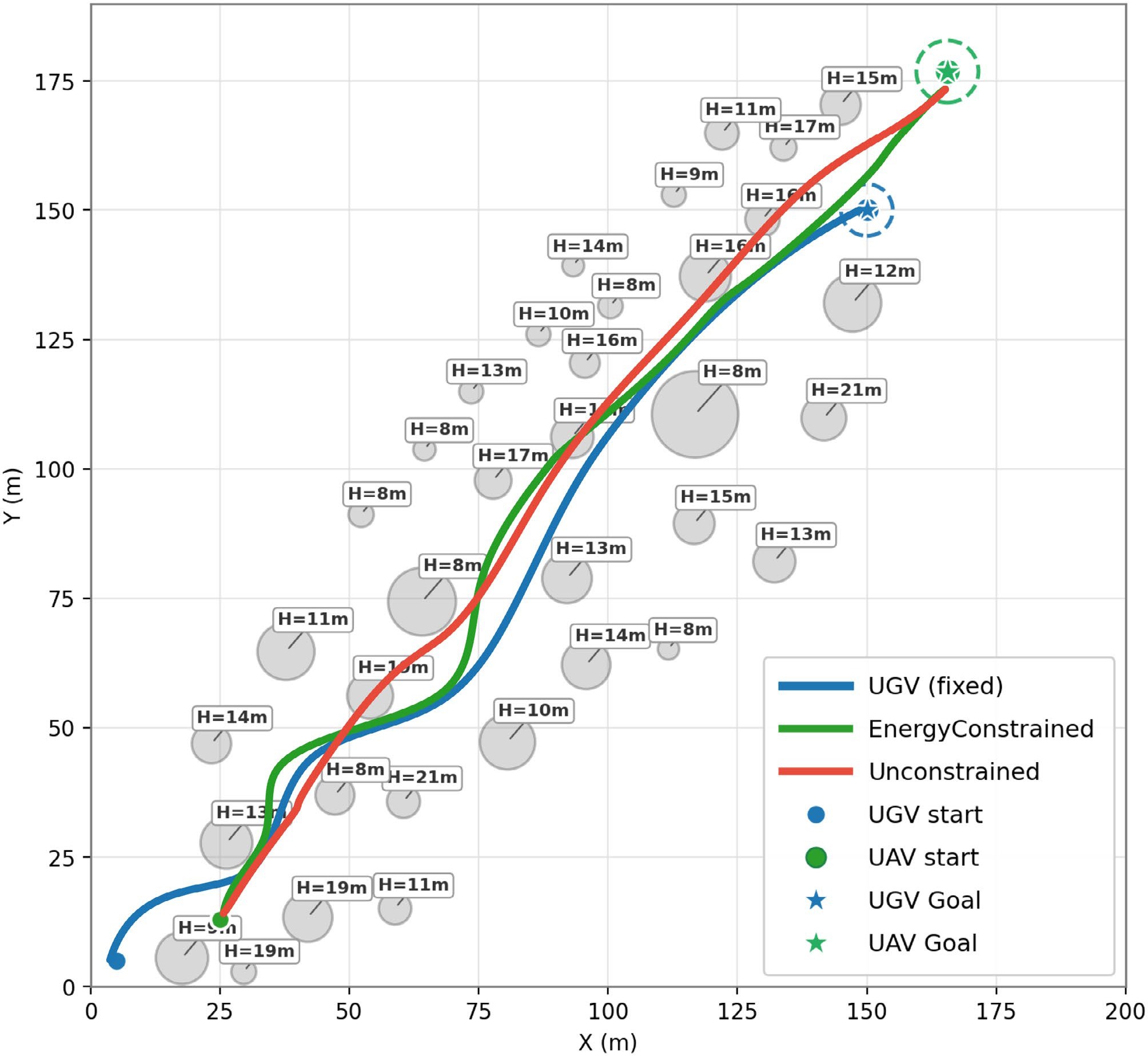
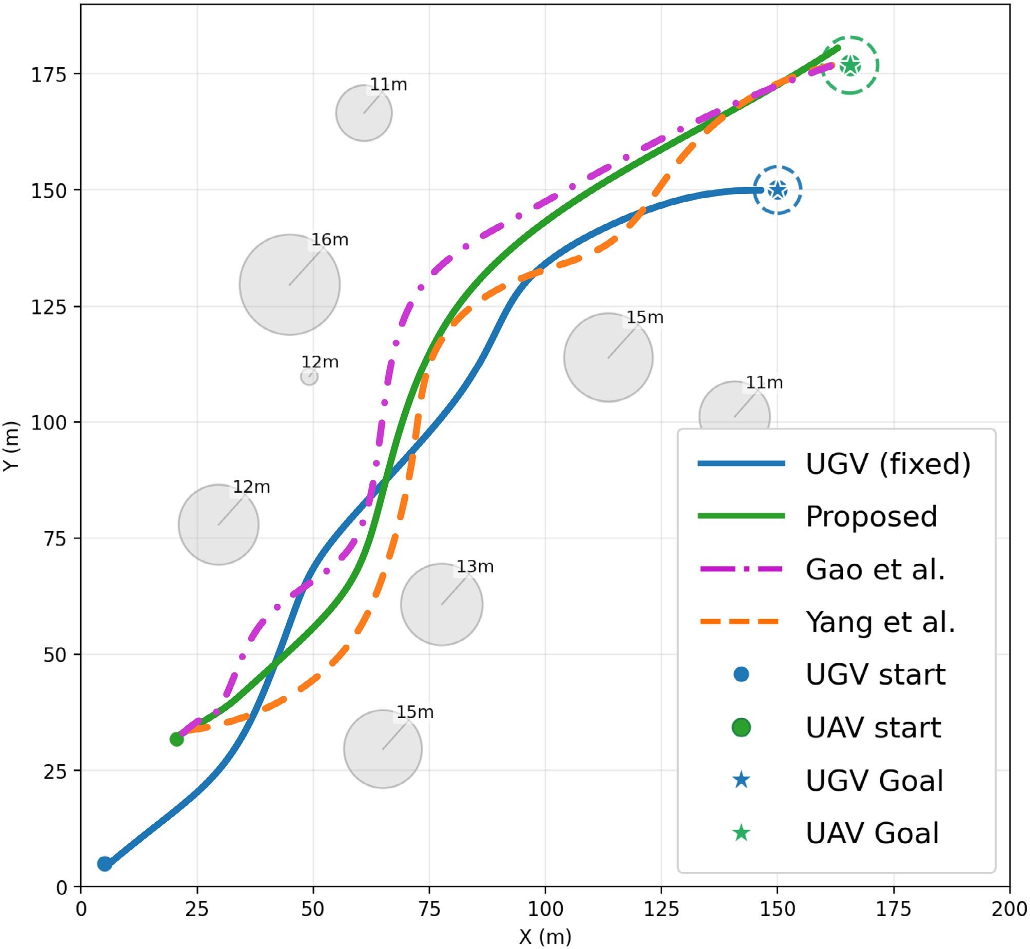
Figure 7.
Scenario 2 (initial LOS): planar trajectories of the UGV and UAV in a cluttered urban environment with multiple obstacles.
-
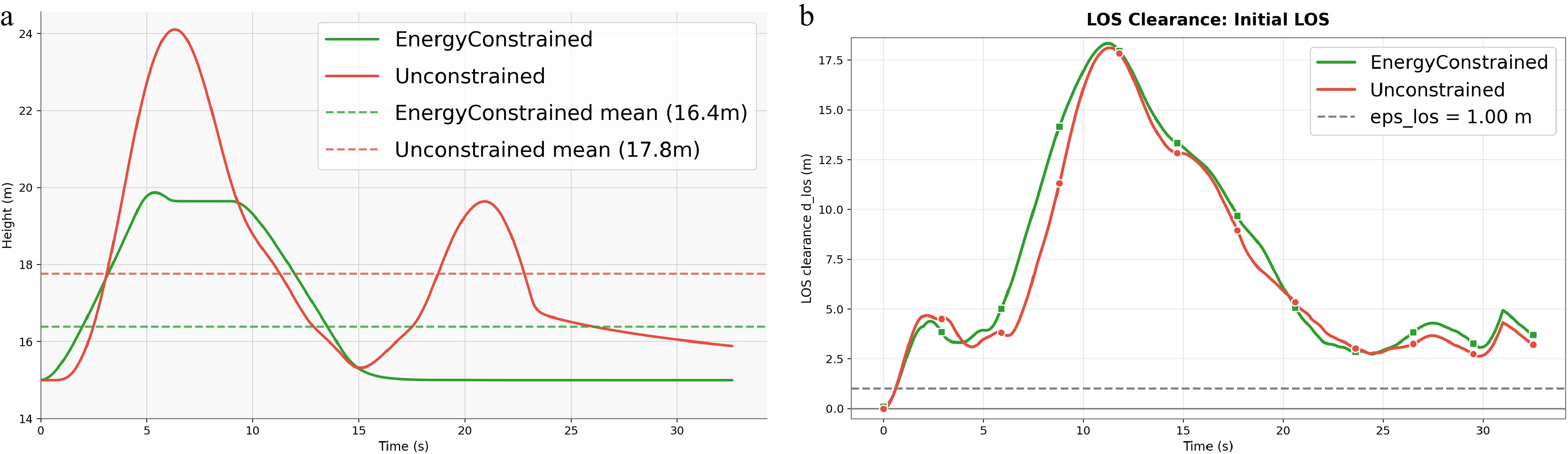
Figure 8.
Scenario 2 (initial LOS): altitude evolution and LOS clearance for Unconstrained and EnergyConstrained. (a) UAV height profiles. (b) LOS clearance/margin metric.
-
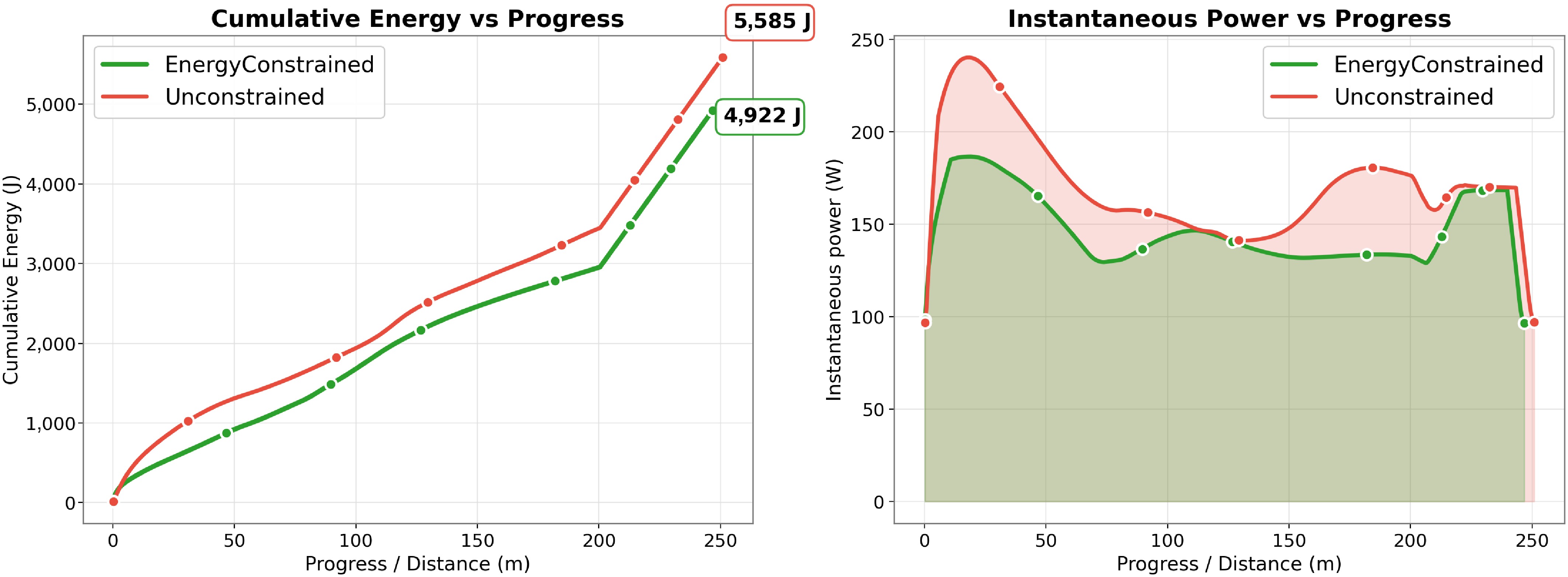
Figure 9.
Scenario 2 (initial LOS): cumulative propulsion energy aligned by progress and instantaneous power computed from executed velocities using Eq. (40).
-
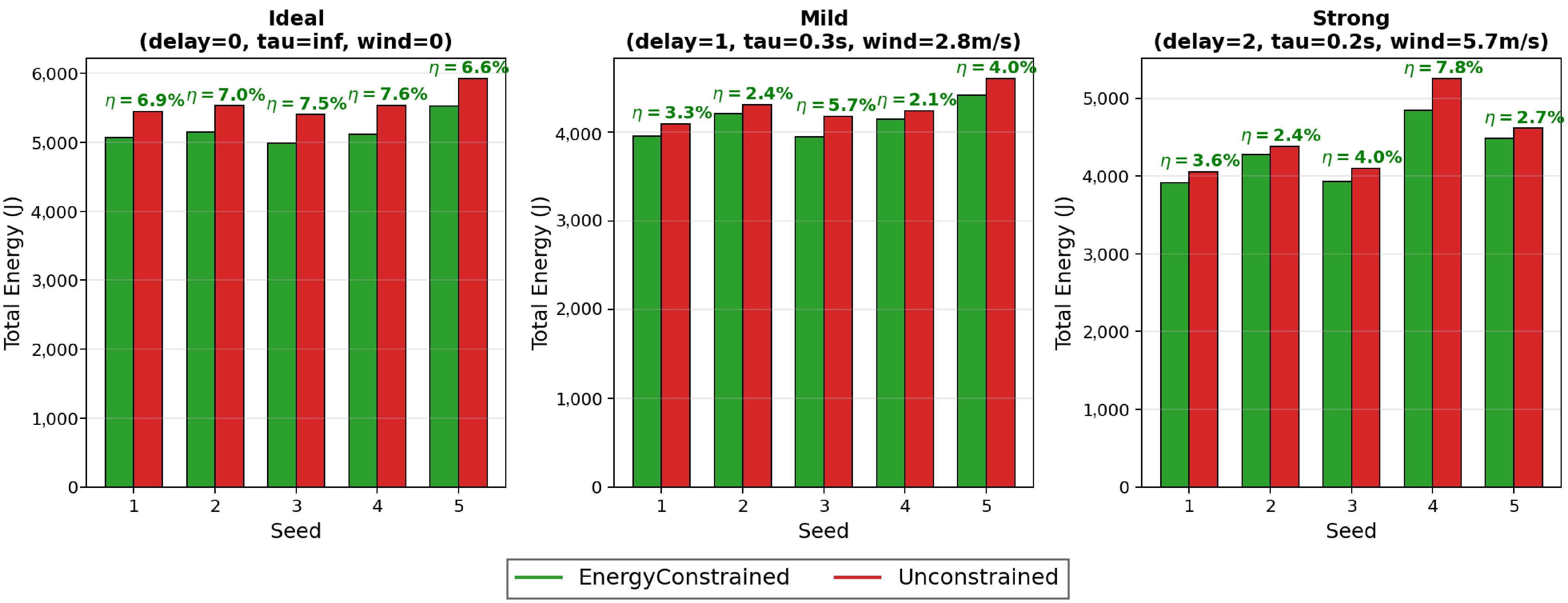
Figure 10.
Energy comparison under ideal, mild-disturbance, and strong-disturbance execution. A positive
$ \eta_E $ -
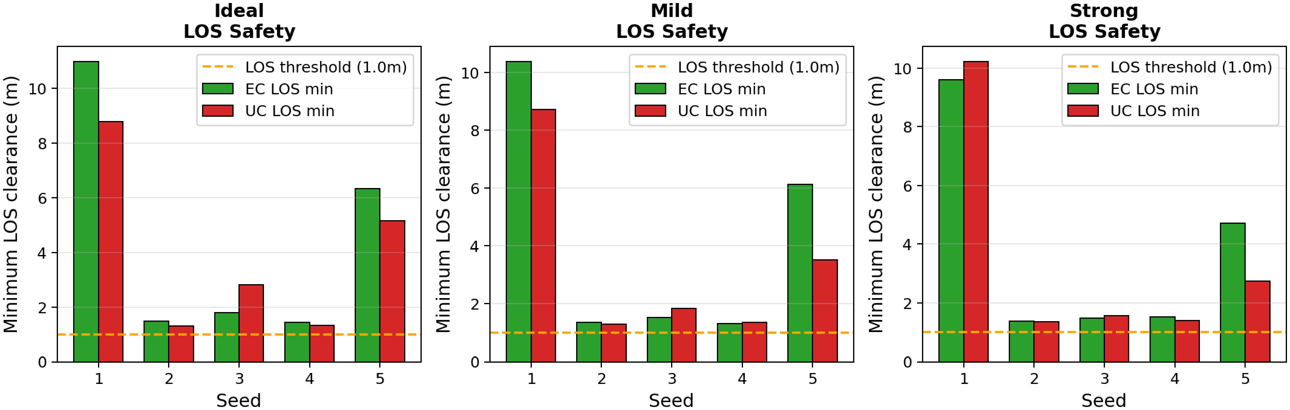
Figure 11.
Minimum LOS clearance under ideal, mild-disturbance, and strong-disturbance execution. The dashed line denotes the LOS safety threshold of 1.0 m.
-
-
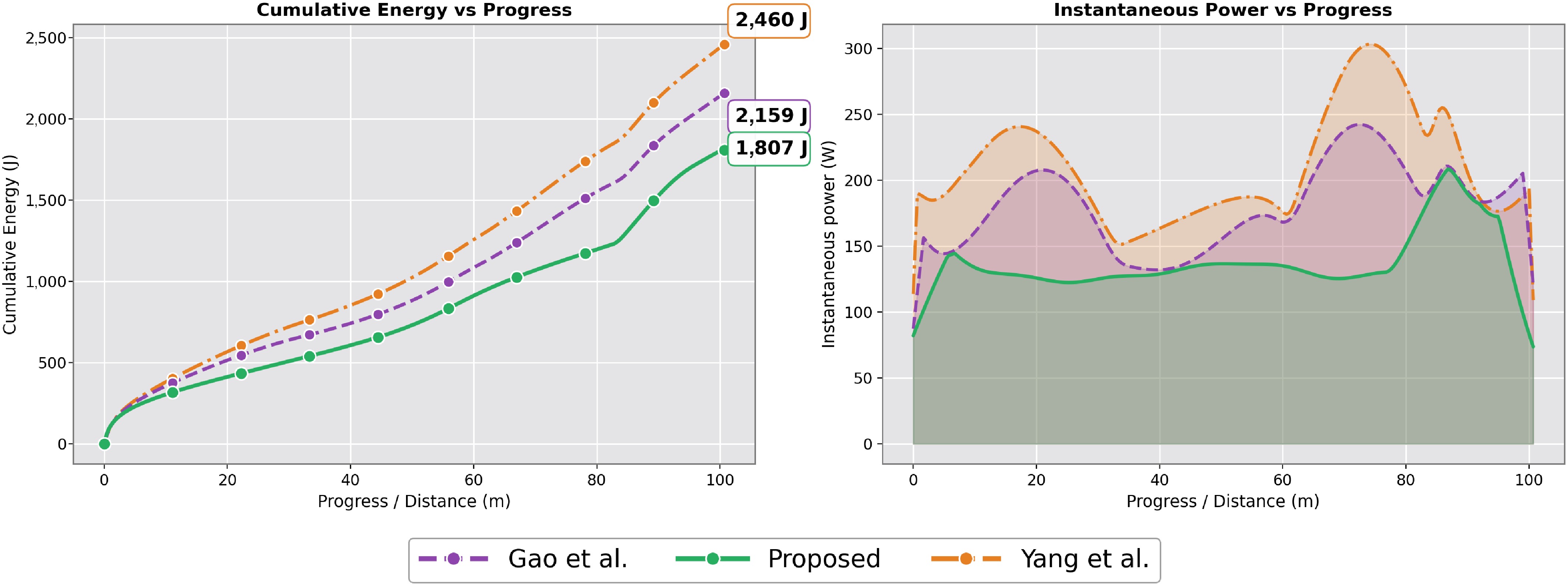
Figure 13.
Progress-aligned cumulative energy and instantaneous power. Cumulative energy is compared at matched UAV progress to reduce bias from different travel distances.
-
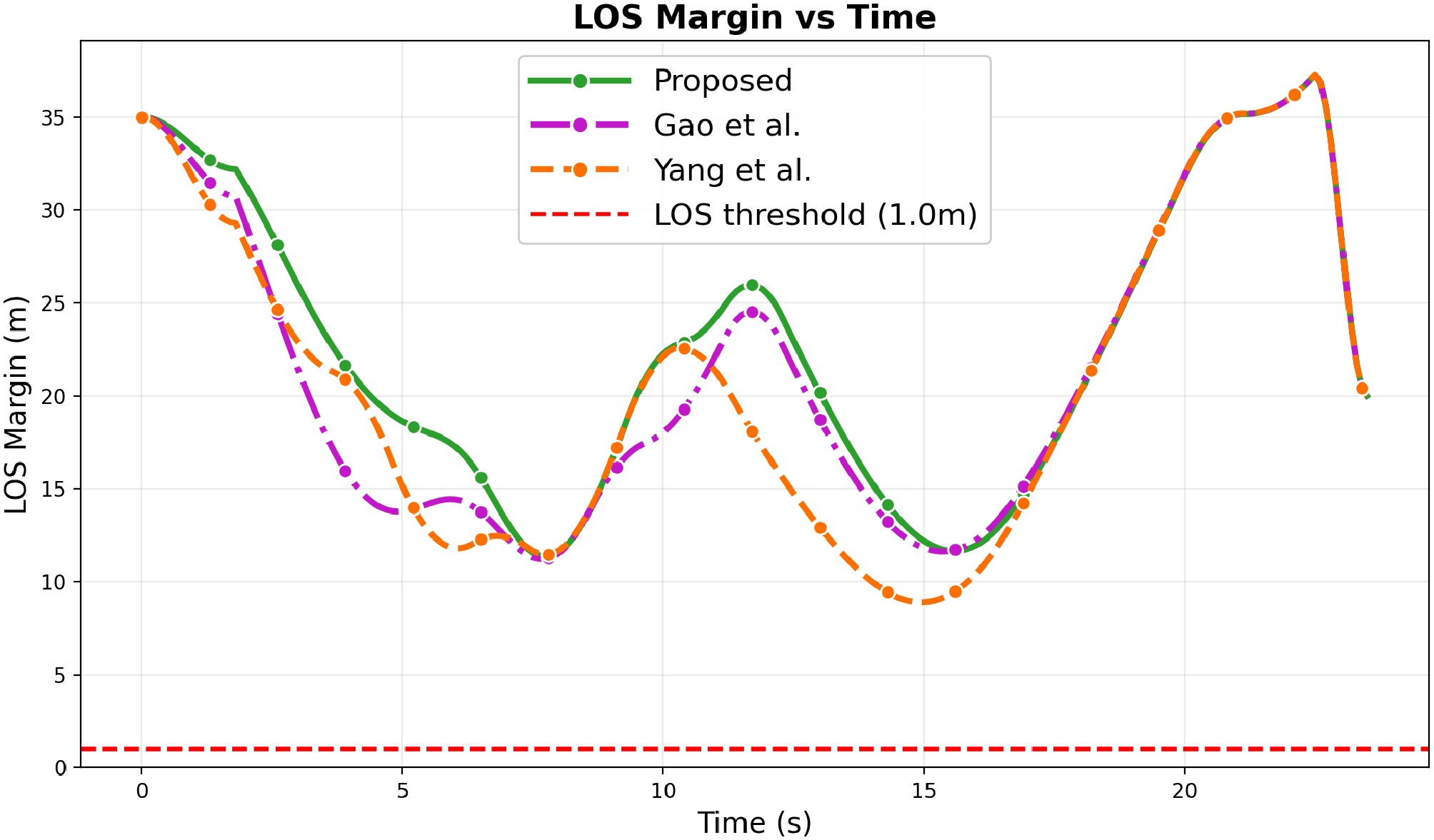
Figure 14.
LOS margin over time under the three embedded propulsion-energy models, with
$ \varepsilon_{\rm{LOS}}=1.0\rm{\ m} $ -
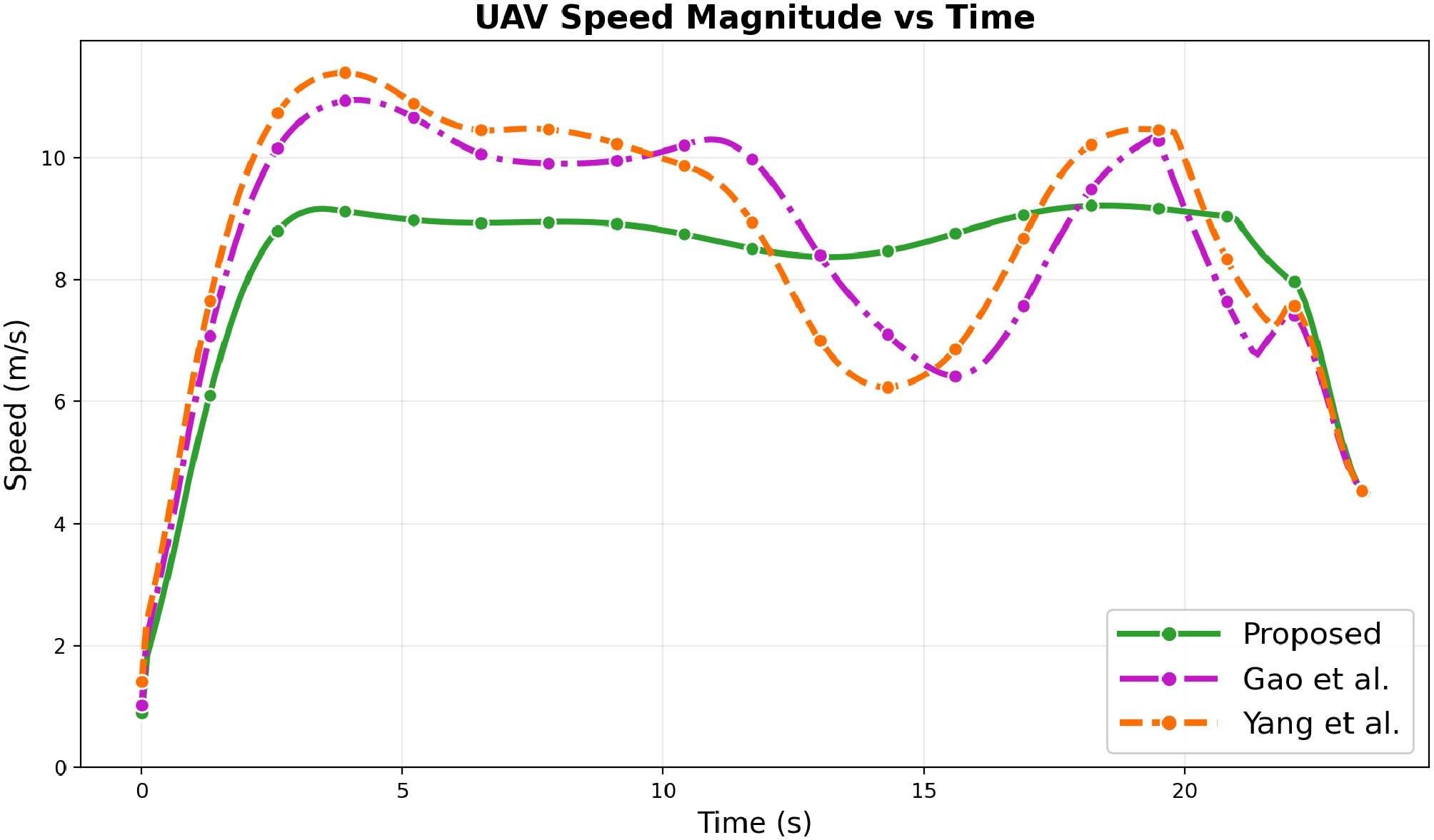
Figure 15.
UAV speed magnitude over time under the three embedded propulsion-energy models.
-
Input: Sampling period $ \Delta t $ $ N_{{\rm{ep}}} $ $ {\cal{O}} $ $ {\rm{UGVRef}}(\cdot) $ $ {\bf{x}}_{v,g} $ $ (S,\tau,\varepsilon_{{\rm{LOS}}}) $ $ (s_{\min},d_{{\rm{ahead}}}) $ $ (v_{\max},v_{z,\max}) $ $ (z_{\min},z_{\max}) $ $ m_{{\rm{col}}} $ $ ({\cal{A}},{\cal{B}},{\cal{G}}) $ $ (\lambda_E,\lambda_{\Delta v}) $ $ (\eta_{{\rm{LOS}}},\eta_{{\rm{obs}}},\eta_f,\eta_v,\eta_{\Delta v}) $ $ \Theta_E $ Output: Learned policy $ \pi_{\theta} $ $ {\cal{S}}(\cdot) $ 1: $ \theta\leftarrow{\rm{Init}}() $ $ {\cal{D}}\leftarrow\emptyset $ 2: for $ {\rm{ep}}=1 $ $ N_{{\rm{ep}}} $ 3: $ ({\bf{x}}_{u,0},{\bf{x}}_{v,0})\leftarrow{\rm{Reset}}() $ $ {\bf{v}}_{{\rm{safe}},-1}\leftarrow\mathbf{0} $ 4: for $ t=0 $ $ T-1 $ 5: $ o_t\leftarrow{\rm{Obs}}({\bf{x}}_{u,t},{\bf{x}}_{v,t}) $ $ {\bf{v}}_{{\rm{des}},t}\sim\pi_{\theta}(\cdot\mid o_t) $ 6: $ {\bf{v}}_{v,t}\leftarrow{\rm{UGVRef}}({\bf{x}}_{v,t},t) $ 7: $ (d_{{\rm{LOS}},t},g_{{\rm{LOS}},t},\hat{{\bf{t}}}_{v,t},s_{f,t}) \leftarrow {\rm{Metrics}}({\bf{x}}_{u,t},{\bf{x}}_{v,t},{\bf{x}}_{v,g},{\cal{O}},b,S,\tau) $ 8: $ {\bf{p}}_{{\rm{ref}},t} \leftarrow {\bf{x}}_{v,t}+d_{{\rm{ahead}}}\hat{{\bf{t}}}_{v,t} $ 9: $ {\cal{C}}_t \leftarrow {\rm{CandidateSet}}({\bf{v}}_{{\rm{des}},t},{\cal{A}},{\cal{B}},{\cal{G}},v_{\max},v_{z,\max}) $ 10: $ (\hat{{\bf{x}}}_{u,t+1},\hat{{\bf{x}}}_{v,t+1}, \hat{d}_{{\rm{obs}},t+1}, \hat{g}_{{\rm{LOS}},t+1}, \hat{s}_{f,t+1}) \leftarrow {\rm{PredictEvaluate}} ({\cal{C}}_t,{\bf{x}}_{u,t},{\bf{x}}_{v,t},{\bf{v}}_{v,t}, {\bf{x}}_{v,g},{\cal{O}},b,S,\tau,\Delta t) $ 11: $ {\cal{V}}_t \leftarrow {\rm{AdmissibleSet}} ({\cal{C}}_t, \hat{{\bf{x}}}_{u,t+1}, \hat{d}_{{\rm{obs}},t+1}, \hat{g}_{{\rm{LOS}},t+1}, \hat{s}_{f,t+1}, z_{\min},z_{\max},m_{{\rm{col}}}, \varepsilon_{{\rm{LOS}}},s_{\min}) $ 12: if $ {\cal{V}}_t\neq\emptyset $ 13: $ {\bf{v}}_{{\rm{safe}},t} \leftarrow {\rm{Project}} ({\cal{V}}_t,{\bf{v}}_{{\rm{des}},t},{\bf{v}}_{{\rm{safe}},t-1}, \lambda_E,\lambda_{\Delta v}) $ 14: else 15: $ {\bf{v}}_{{\rm{safe}},t} \leftarrow {\rm{Recover}} ({\cal{C}}_t, \hat{g}_{{\rm{LOS}},t+1}, \hat{d}_{{\rm{obs}},t+1}, \hat{s}_{f,t+1}, {\bf{v}}_{{\rm{safe}},t-1}, \eta_{{\rm{LOS}}},\eta_{{\rm{obs}}},\eta_f,\eta_v,\eta_{\Delta v}) $ 16: end if 17: $ {\bf{x}}_{u,t+1} \leftarrow {\bf{x}}_{u,t}+{\bf{v}}_{{\rm{safe}},t}\Delta t $ $ {\bf{x}}_{v,t+1} \leftarrow {\bf{x}}_{v,t}+{\bf{v}}_{v,t}\Delta t $ 18: $ I_t\leftarrow \|{\bf{v}}_{{\rm{safe}},t}-{\bf{v}}_{{\rm{des}},t}\|_2 $ $ E_t\leftarrow {\rm{Energy}}({\bf{v}}_{{\rm{safe}},t};\Theta_E)\Delta t $ 19: $ (\hat{{\bf{t}}}_{v,t+1},s_{f,t+1}) \leftarrow {\rm{Ahead}}({\bf{x}}_{u,t+1},{\bf{x}}_{v,t+1},{\bf{x}}_{v,g}) $ $ {\bf{p}}_{{\rm{ref}},t+1} \leftarrow {\bf{x}}_{v,t+1}+d_{{\rm{ahead}}}\hat{{\bf{t}}}_{v,t+1} $ 20: $ r_{{\rm{prog}},t} \leftarrow \|{\bf{x}}_{u,t}-{\bf{p}}_{{\rm{ref}},t}\|_2 - \|{\bf{x}}_{u,t+1}-{\bf{p}}_{{\rm{ref}},t+1}\|_2 $ 21: $ \sigma_{{\rm{blk}},t} \leftarrow [\varepsilon_{{\rm{LOS}}}-g_{{\rm{LOS}},t}]_{+} $ $ \sigma_{f,t}\leftarrow[s_{\min}-s_{f,t}]_{+} $ 22: $ r_t \leftarrow {\rm{Reward}} (r_{{\rm{prog}},t},E_t,I_t,\sigma_{{\rm{blk}},t},\sigma_{f,t}, {\bf{v}}_{{\rm{safe}},t},{\bf{v}}_{{\rm{safe}},t-1};w) $ 23: $ o_{t+1}\leftarrow{\rm{Obs}}({\bf{x}}_{u,t+1},{\bf{x}}_{v,t+1}) $ 24: $ {\cal{D}}\leftarrow {\cal{D}}\cup \{(o_t,{\bf{v}}_{{\rm{des}},t},{\bf{v}}_{{\rm{safe}},t},r_t,o_{t+1})\} $ 25: $ \theta\leftarrow{\rm{Update}}(\theta,{\cal{D}},\gamma) $ 26: end for 27: end for 28: return $ \pi_{\theta} $ $ {\cal{S}}(\cdot) $ Table 1.
Energy-efficient constraint-consistent shielded reinforcement learning.
-
Symbol Meaning Value $ \Delta t $ Sampling period $ 0.1 {\rm{s}} $ T Episode horizon 5,000 steps $ L\times W $ Workspace size in $ xy $ 200 m × 180 m $ v_{\max} $ UAV speed limit 15 m/s $ [z_{\min},z_{\max}] $ UAV altitude bounds [5, 30] m $ z_0 $ Initial UAV altitude 15 m $ d_{{\rm{ahead}}} $ Look-ahead reference distance 30 m $ s_{\min} $ Minimum ahead distance 4 m $ \varepsilon_{{\rm{LOS}}} $ LOS margin threshold 1.0 m S LOS samples on the segment 64 τ Soft-min temperature 0.25 $ (d_{{\rm{safe}}},d_{{\rm{crit}}},p) $ LOS risk mapping parameters (1.0 m, 0.2 m, 2) $ m_{{\rm{col}}} $ Collision margin 0.3 m The only difference between EnergyConstrained and Unconstrained is the energy weight $ w_E $ $ w_E>0 $ $ w_E=0 $ Table 1.
Key parameters for the propulsion-energy ablation study.
-
Table 2.
Comparison of three embedded propulsion-energy models under identical task settings and feasibility enforcement.
-
Component Mean (ms) Std. (ms) 95th Perc. (ms) LOS evaluation 11.59 1.86 15.16 ESDF field query 0.17 0.05 0.23 Field-gradient query 0.16 0.04 0.21 Candidate-direction search 11.69 1.95 15.33 Shield mapping 9.99 5.04 15.71 Total per-step time 33.60 7.56 46.76 Table 3.
Online timing breakdown of the proposed SAC–Shield controller under
$ N=15 $ $ S=64 $ -
Setting N S Mean time (ms) Frequency (Hz) Small 5 16 2.75 363.69 Moderate 10 64 17.00 58.82 Default-scale 15 64 22.02 45.41 Large 20 128 58.53 17.08 Largest tested 30 128 86.53 11.56 Table 4.
Scalability of online feasibility evaluation with respect to local obstacles N and LOS samples S.
Figures
(15)
Tables
(5)