-
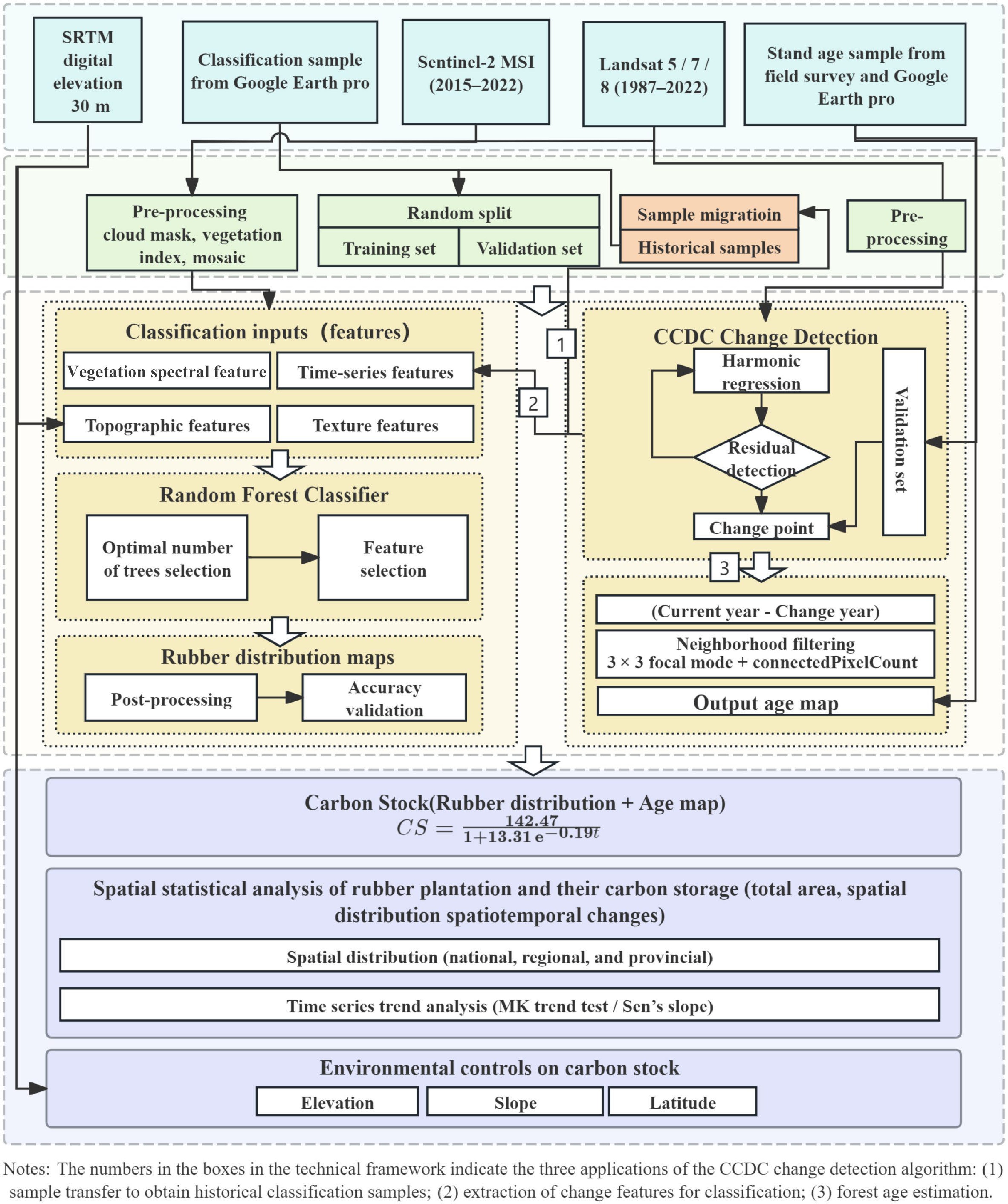
Figure 1.
Workflow of the present study.
-
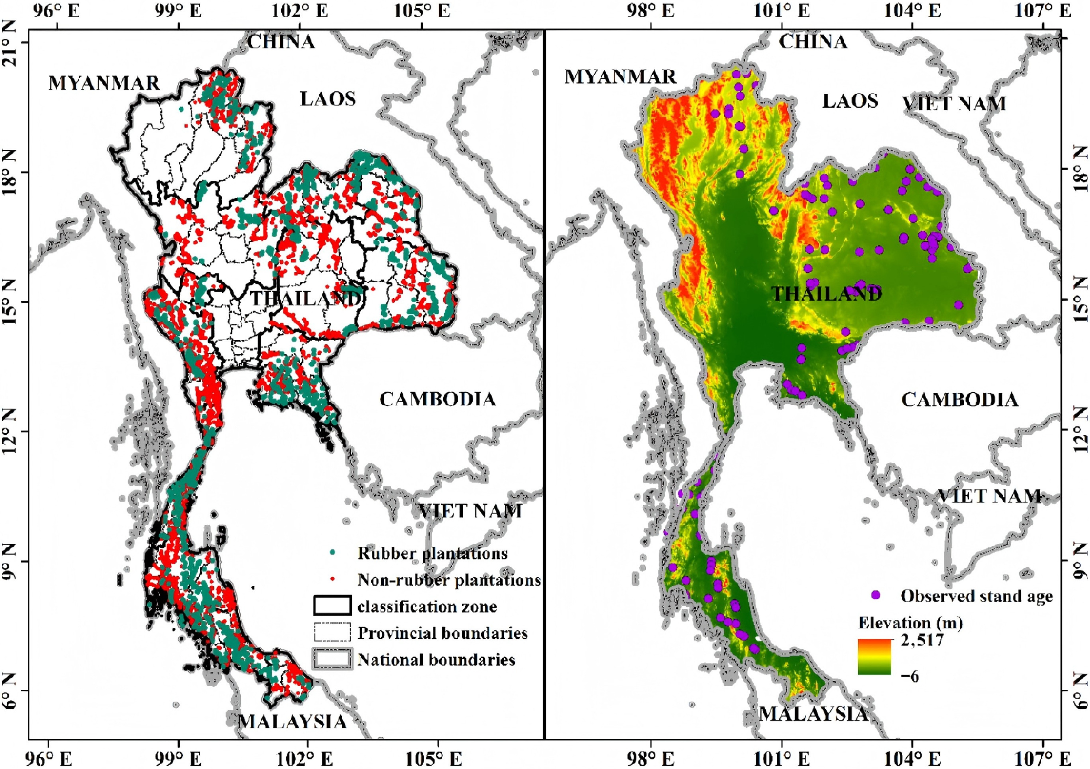
Figure 2.
Map of the study area: (a) Samples (rubber and non-rubber) and classification zones. (b) Stand age sample points and elevation.
-
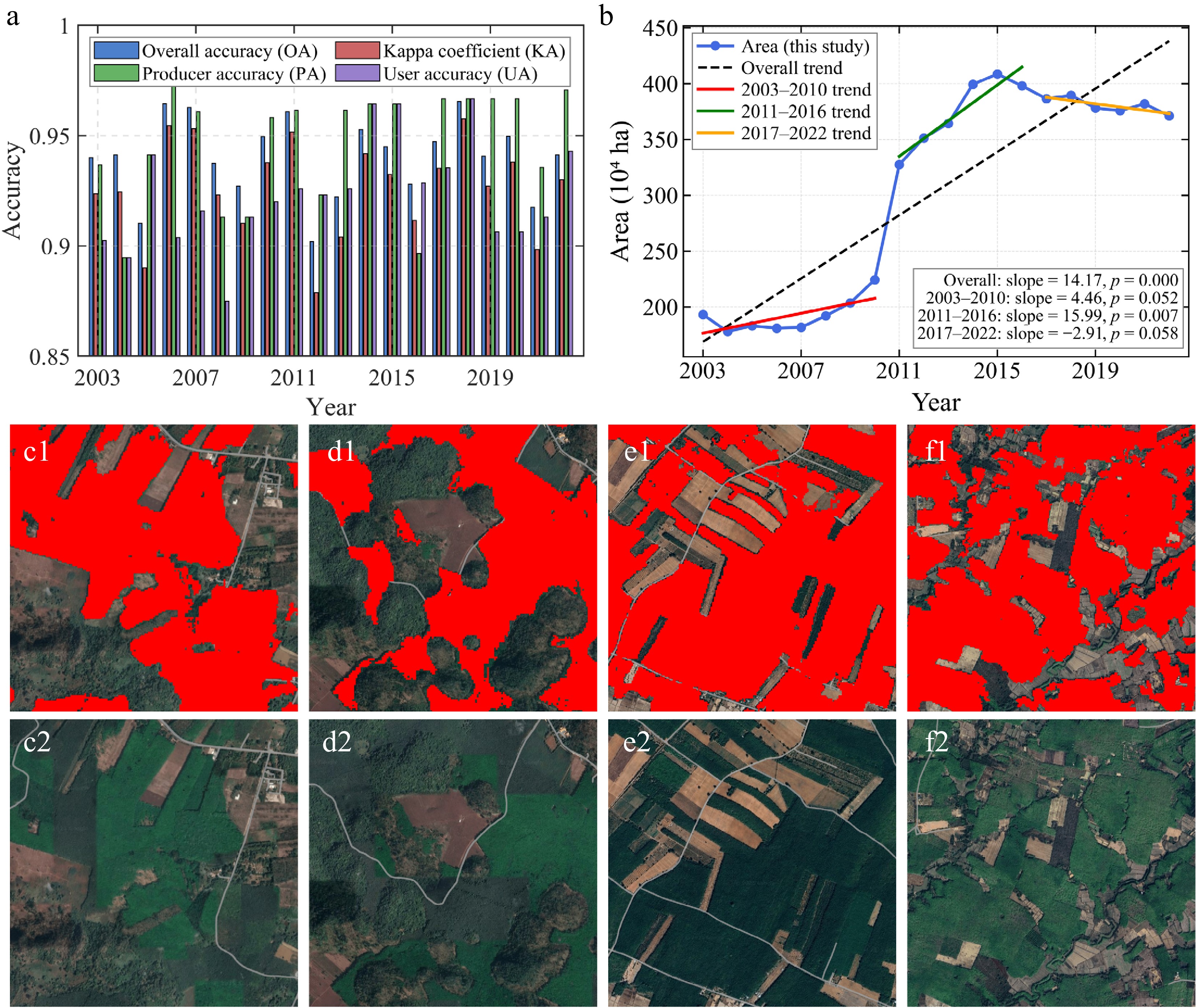
Figure 3.
Rubber classification results: (a) Classification accuracy from 2003 to 2022. (b) Time series of rubber plantation area. (c)−(f) Examination of classified rubber plantations with Google Earth images (2022).
-
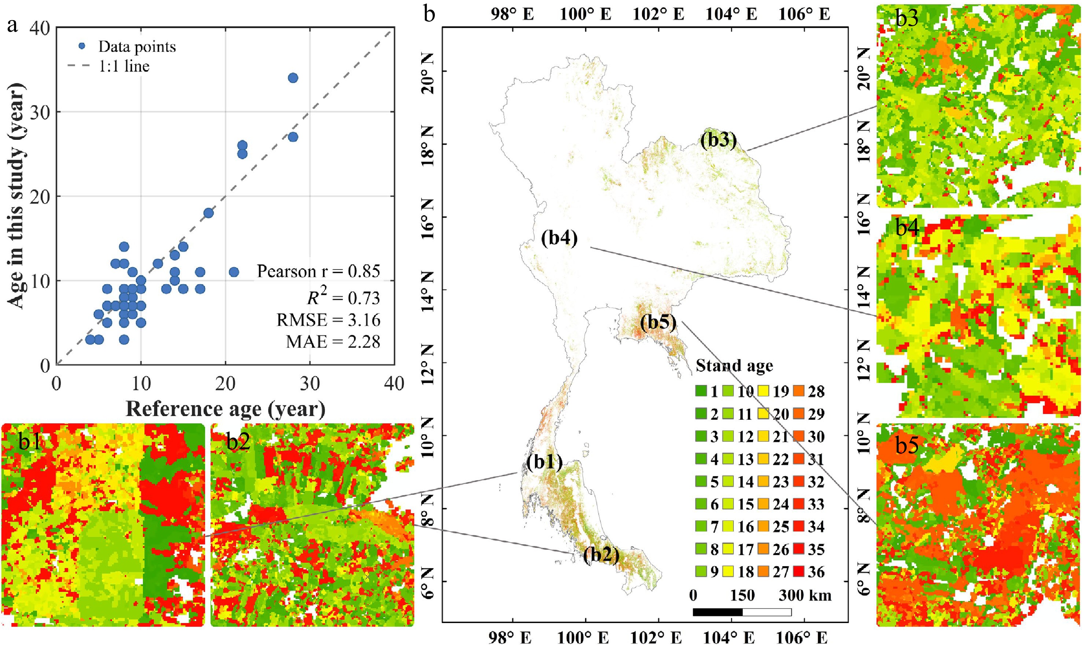
Figure 4.
Stand age results: (a) Stand age validation scatter plot. (b) The retrieved stand age distribution of the year 2022. (b1)–(b5) Zoom areas randomly selected.
-
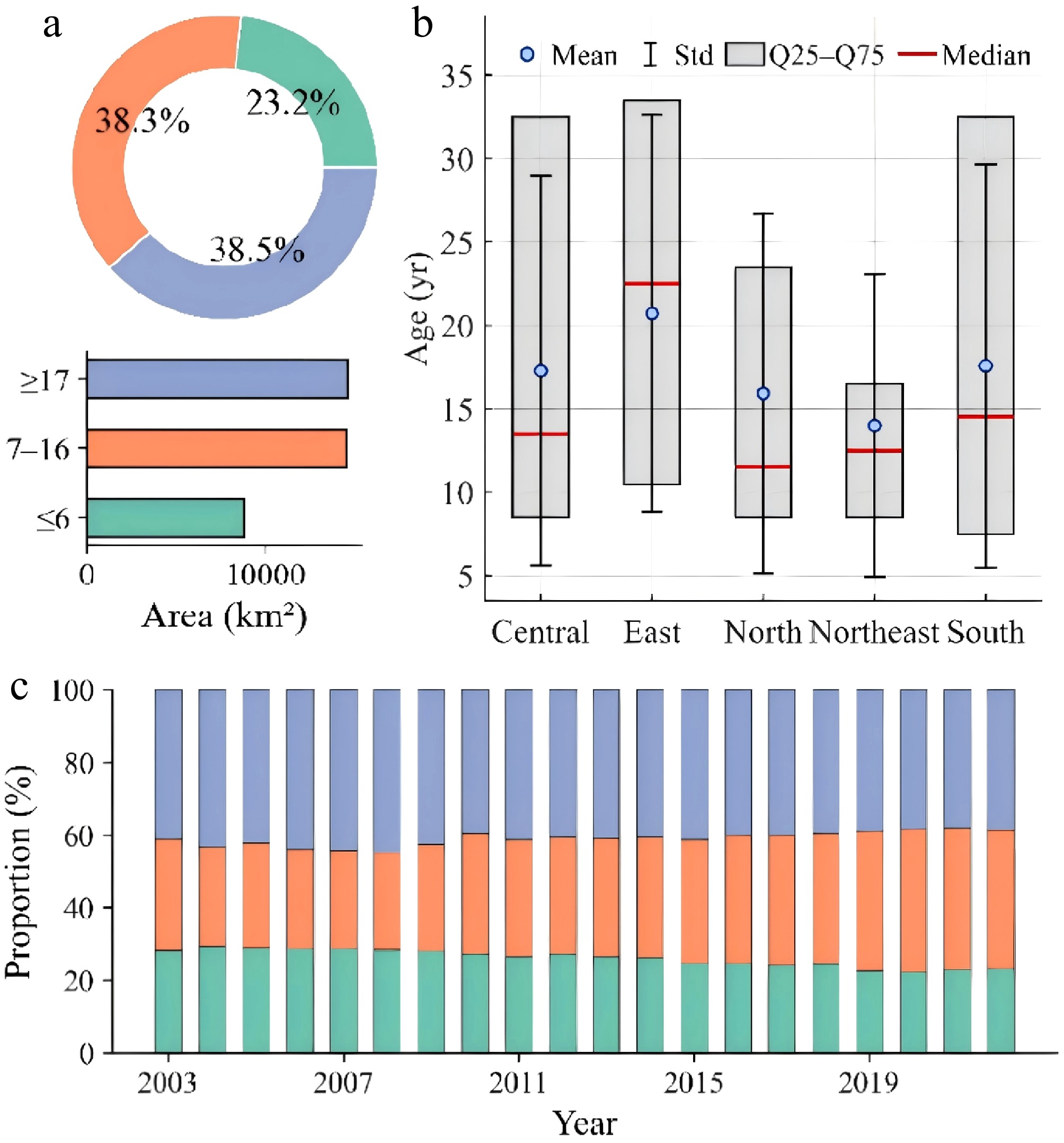
Figure 5.
Stand age statistics: (a) Stand age statistics by region. (b) Stand age stage and the area of each age in 2022. (c) Temporal dynamics of stand age stage from 2003 to 2022.
-
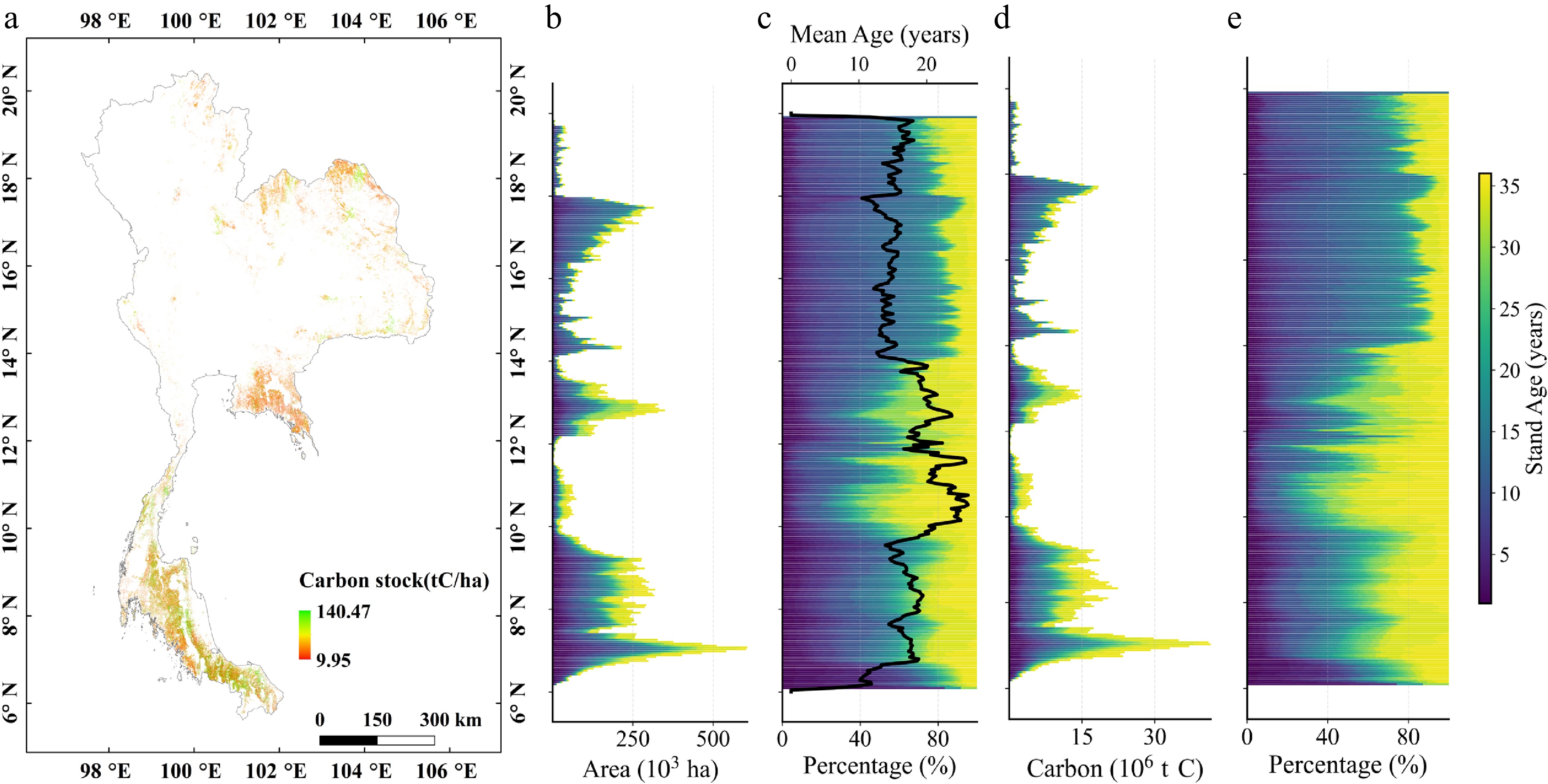
Figure 6.
Carbon stock distribution characteristics: (a) Spatial distribution of carbon stock in 2022. (b) Area of different age variations along the latitudinal gradient. (c) Area percentage of different ages and mean stand age along the latitudinal gradient. (d) Carbon stock of different age variations along the latitudinal gradient. (e) Carbon stock percentage of different ages along the latitudinal gradient.
-
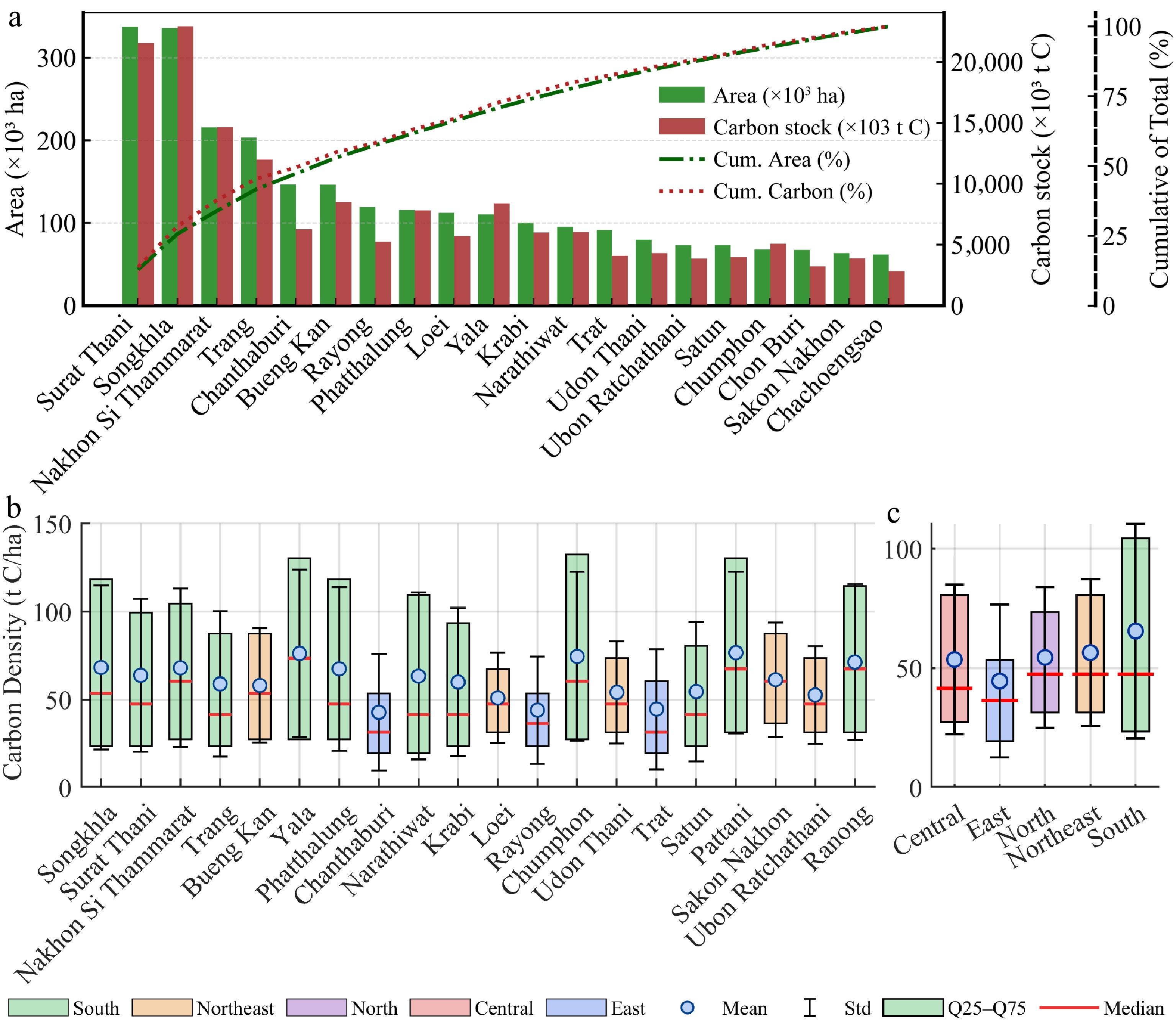
Figure 7.
Regional statistics on carbon stock (2022): (a) Distribution of rubber area and carbon stock by province (top 20 provinces). (b) Carbon density by province (top 20 provinces). (c) Carbon density in each region.
-
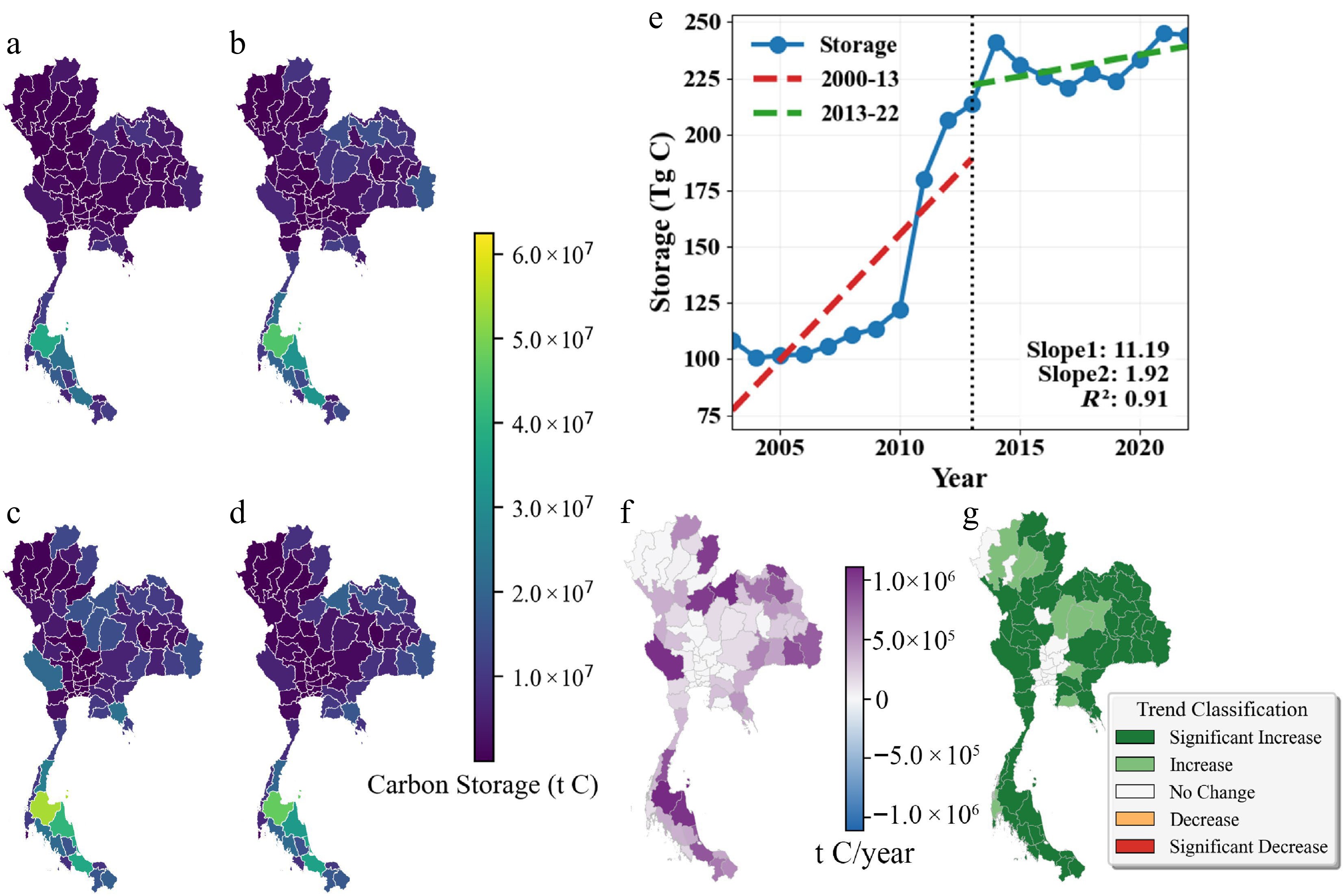
Figure 8.
Spatiotemporal dynamics of carbon stock from 2003 to 2022: (a)−(d) Provincial carbon stock in 2003, 2010, 2016, and 2022. (e) Temporal trends of carbon stock at national and regional scales. (f) Trend magnitude (Sen's slope). (g) Trend significance (Mann–Kendall test).
-
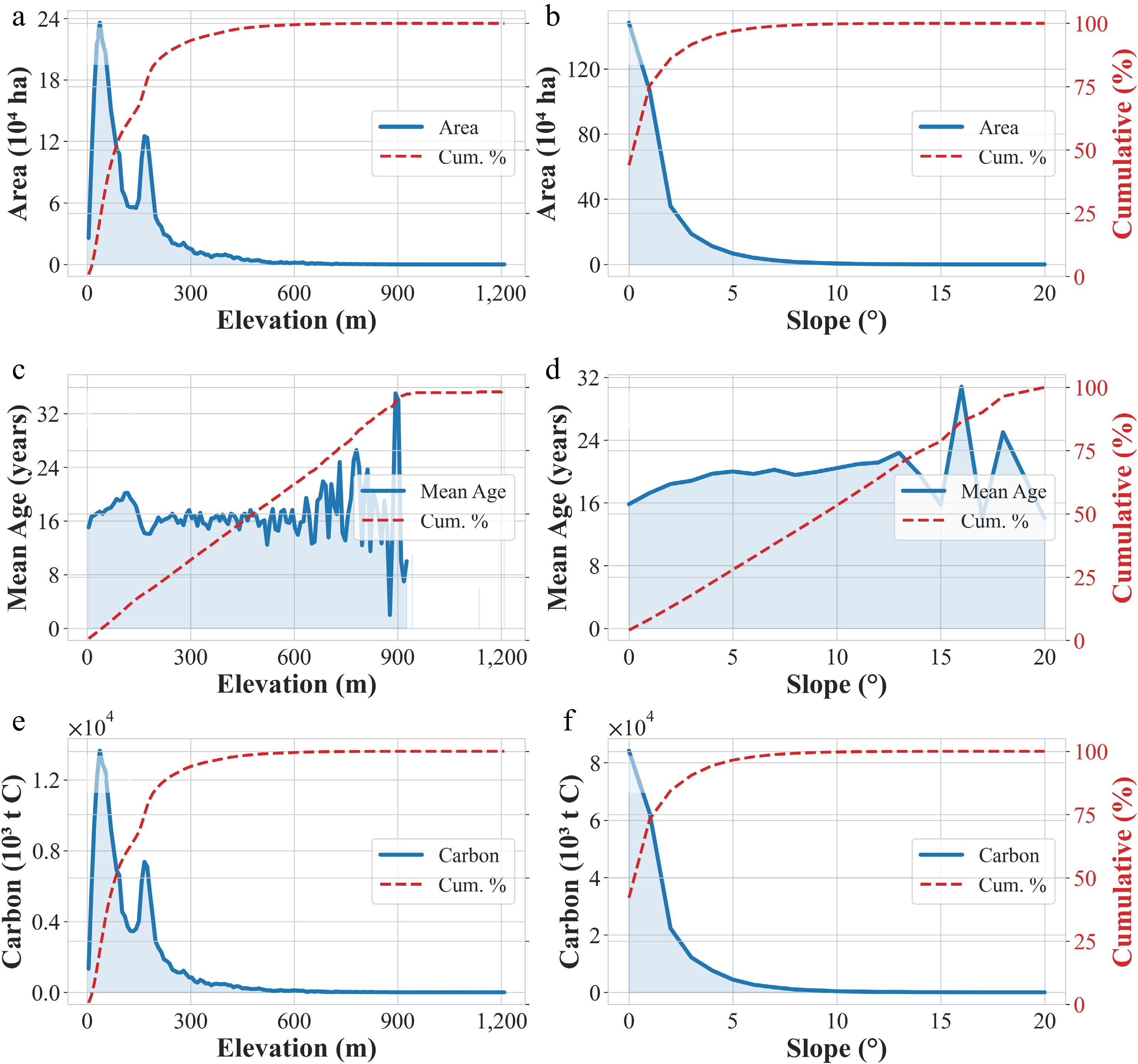
Figure 9.
Planted area and carbon stock variations along topography: (a)−(f) Changes in planting area, carbon stock, and forest age across elevation ranges and slope regions.
-
Dataset Description Period Source USGS/SRTMGL1_003 Global DEM with 30 m spatial resolution; used for terrain analysis (slope, aspect). ~2000 https://developers.google.com/earth-engine/datasets/catalog/USGS_SRTMGL1_003 LANDSAT/LC08/C02/T1_L2 Landsat 8 surface reflectance (30 m, 16-d revisit); for large-area classification and change detection. 2013−2022 https://developers.google.com/earth-engine/datasets/catalog/LANDSAT_LC08_C02_T1_L2 LANDSAT/LE07/C02/T1_L2 Landsat 7 surface reflectance (30 m, 16-d revisit); for land-cover analysis and change detection. 1999−2022 https://developers.google.com/earth-engine/datasets/catalog/LANDSAT_LE07_C02_T1_L2 LANDSAT/LT05/C02/T1_L2 Landsat 5 surface reflectance (30 m, 16-d revisit); for long-term change monitoring. 1984−2011 https://developers.google.com/earth-engine/datasets/catalog/LANDSAT_LT05_C02_T1_L2 COPERNICUS/S2 & S2_SR_HARMONIZED Sentinel-2 multispectral imagery (10−20 m, 5-d revisit); includes Level-1C (TOA reflectance) and Level-2A (surface reflectance, harmonized). Used for vegetation, soil, and urban feature monitoring. 2015−2022 https://developers.google.com/earth-engine/datasets/catalog/COPERNICUS_S2_SR_HARMONIZED High-resolution classification samples Rubber polygons digitized from high-resolution imagery for classification. Google Earth Pro Rubber stand ages in Thailand Field survey rubber plots. [42] Table 1.
Data used in this study.
-
Feature group Variable (abbr.) Definition/description Ref. Spectral Bands (B) Blue, Green, Red, NIR, SWIR1, SWIR2 NDVI, NDVImin/mean/max $ \dfrac{\text{NIR}-\text{RED}}{\text{NIR}+\text{RED}} $ [44] NDBI $ \dfrac{\mathrm{SWIR}1-\text{NIR}}{\mathrm{SWIR}1+\text{NIR}} $ [45] NDMI $ \dfrac{\text{NIR}-\text{SWIR}2}{\text{NIR}+\text{SWIR}2} $ [43] MNDWI $ \dfrac{\text{GREEN}-\text{SWIR}1}{\text{GREEN}+\text{SWIR}1} $ [46] NBR $ \dfrac{\text{NIR}-\text{SWIR}1}{\text{NIR}+\text{SWIR}1} $ [47] EVI $ 2.5\times \dfrac{\text{NIR}-\text{RED}}{\text{NIR}+6\text{RED}-7.5\text{BLUE}+1} $ [48] Phenology EVI_Jan (EVIj), EVI_Feb (EVIf), EVI_Mar (EVIm) Monthly EVI composites for Jan–Mar [41] Texture SAVG, ENT, ASM, IDM GLCM sum average, entropy, angular second moment, inverse difference moment [43] Change detection RMSE, DensityObs, Mag Root-mean-square error, observation density, maximum amplitude [33] Terrain Elevation, aspect, slope Elevation, aspect, slope [49] Note: RED, BLUE, NIR, SWIR1, and SWIR2 denote reflectance in the red, blue, near-infrared, shortwave-infrared 1, and shortwave-infrared 2 bands, respectively. Table 2.
Variable set used for key variable selection in this study.
-
Class W IPV RP OP CR NRF Shrub Total UA (%) W 228 0 0 0 4 0 3 235 97.02 IPV 0 168 0 0 2 0 0 170 98.82 RP 4 0 401 9 4 11 12 441 90.93 OP 0 0 8 222 2 5 0 237 93.67 CR 12 2 2 3 228 4 2 253 90.12 NRF 0 0 10 3 6 302 14 335 90.15 Shrub 0 0 12 2 5 9 140 168 83.33 Total 244 170 433 239 251 331 171 1,839 PA (%) 93.44 98.82 92.61 92.89 90.84 91.24 81.87 OA (%) 92.63 Kappa 0.91 F1 score (%) 92.75 Note: W = Water; IPV = Impervious; RP = Rubber Plantation; OP = Oil Palm; CR = Cropland; NRF = Non-Rubber Forest. Table 3.
National scale confusion matrix of the classification result in 2022.
Figures
(9)
Tables
(3)