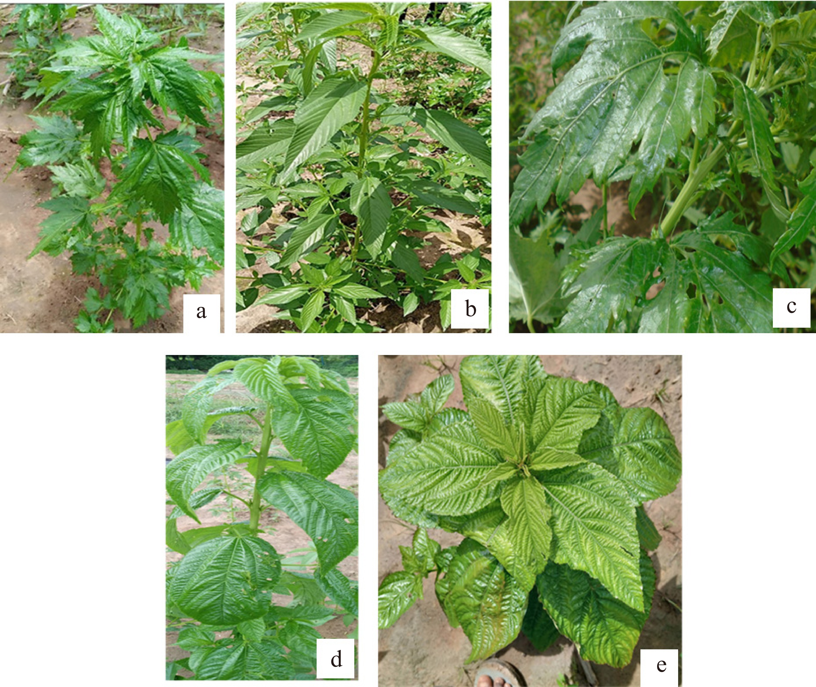
Agronomic performance, genotype x environment interaction, and stability of leaf yield of Jute mallow (<i>Corchorus olitorius</i> L.) in Burkina Faso

Figures (4) Tables (11)

Figure 1.
Characteristics of some genotypes and two varieties used in this study.
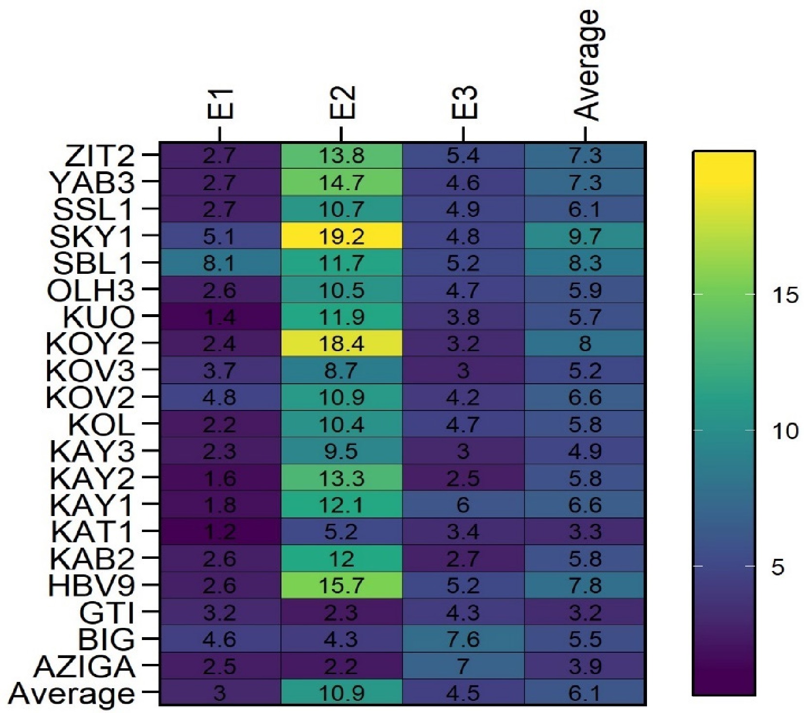
Figure 2.
Heat map illustrating the average yield of genotypes across three locations to visually assess G × E interactions: Ouahigouya (E1), Gampela (E2), and Sogossagasso (E3).
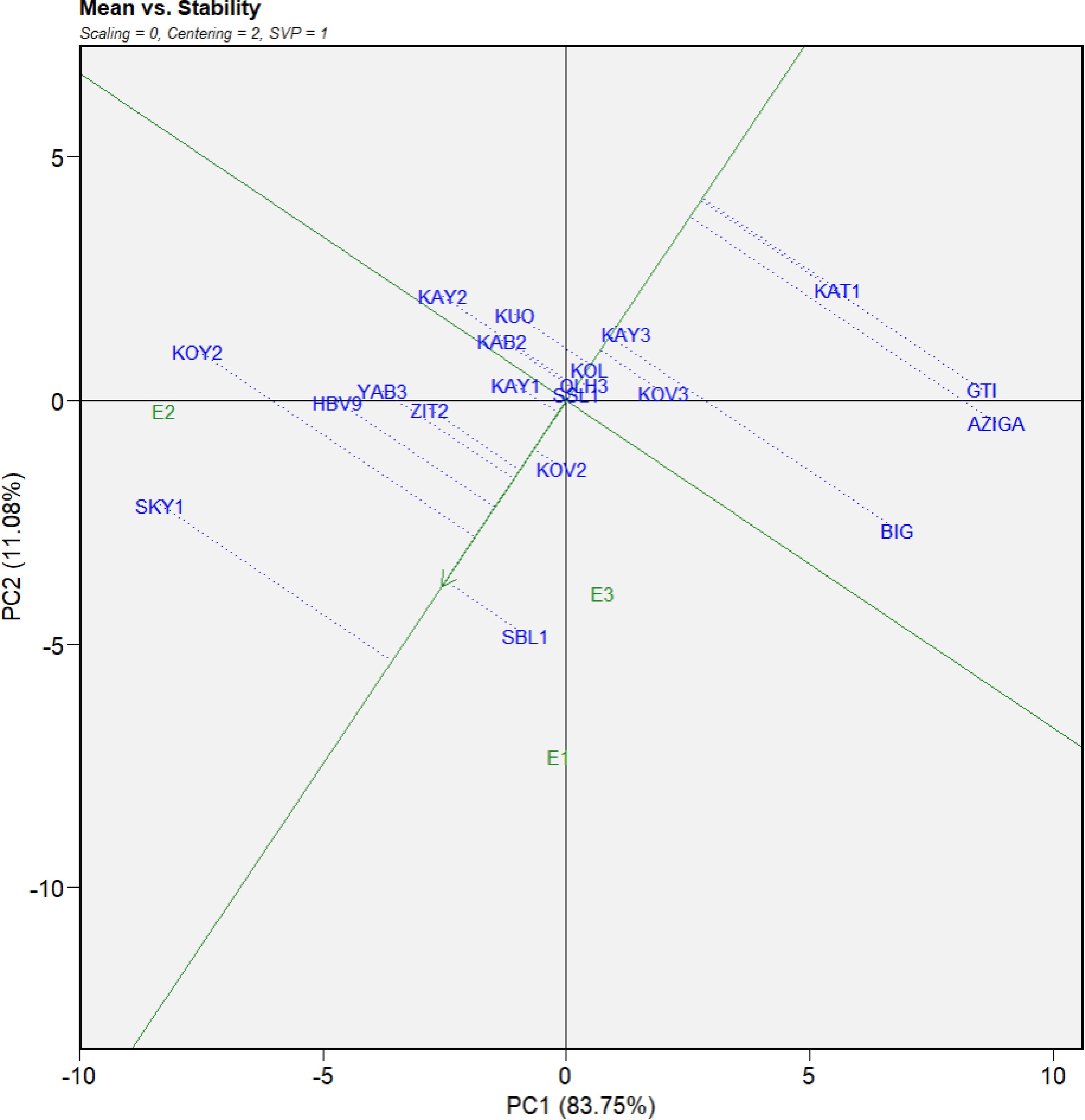
Figure 3.
The ranking biplot shows the mean performance and stability of 20 Jute mallow (C. olitorius) genotypes across three locations: Ouahigouya (E1), Gampela (E2), Sogossagasso (E3).
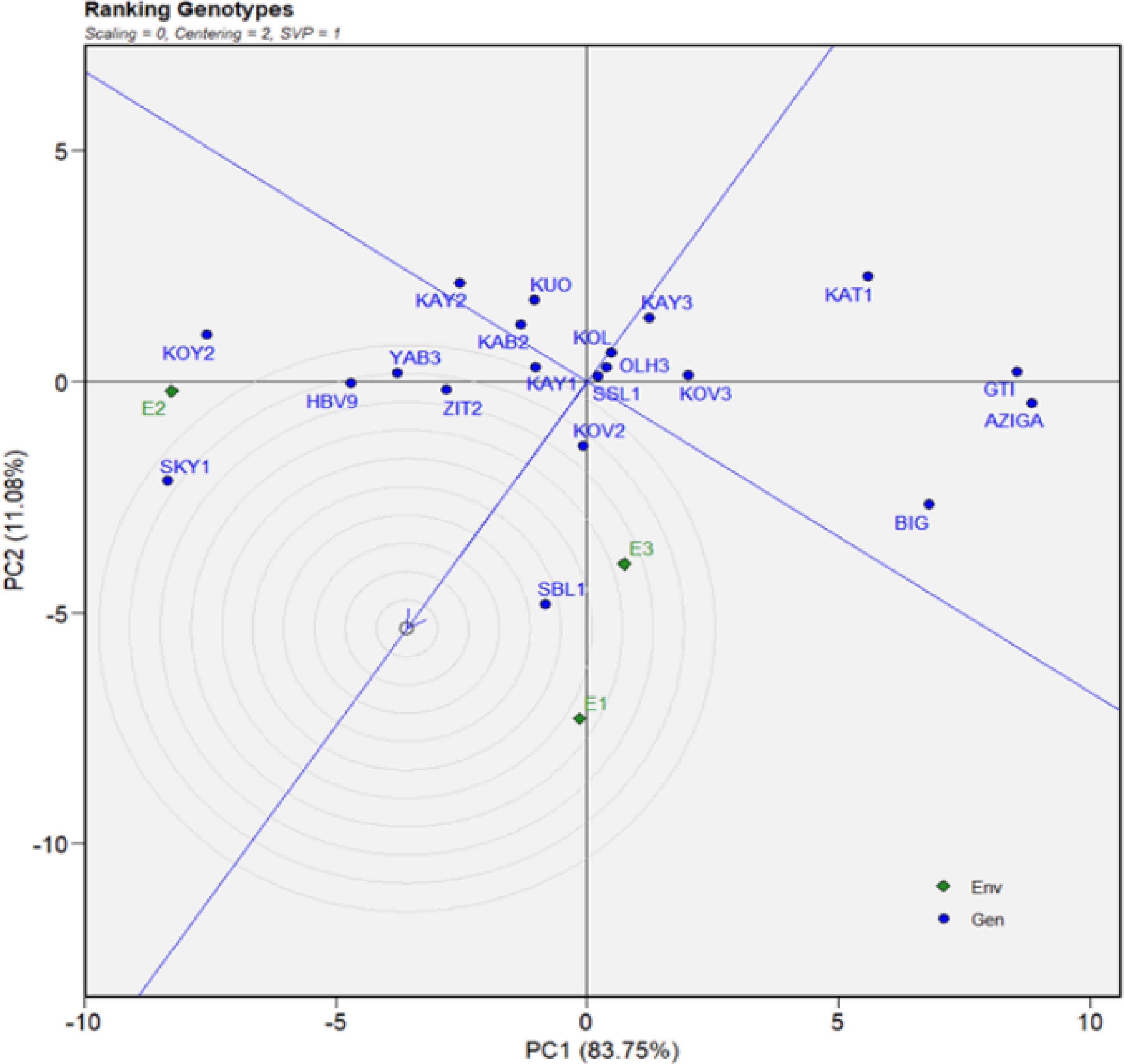
Figure 4.
GGE-biplot showing the ideal genotypes. Ouahigouya (E1), Gampela (E2), Sogossagasso (E3), genotype (Gen), and environment (Env).

Code	Origin	Genotypic characteristics (leaves)
AZIGA	Worldveg	Ovate lanceolate, glossy leaf surface
BIG	Worldveg	Ovate, glossy leaf surface
GTI	Burkina Faso	Ovate
HBV9	Burkina Faso	Palmate, glossy leaf surface
KAB2	Burkina Faso	Palmate
KAT1	Burkina Faso	Palmate
KAY1	Burkina Faso	Palmate
KAY2	Burkina Faso	Palmate
KAY3	Burkina Faso	Palmate
KOL	Burkina Faso	Lanceolate
KOV2	Burkina Faso	Palmate
KOV3	Burkina Faso	Palmate
KOY2	Burkina Faso	Palmate
KUO	Burkina Faso	Palmate
OLH3	Burkina Faso	Palmate
SBL1	Burkina Faso	Palmate, glossy leaf surface
SKY1	Burkina Faso	Palmate
SSL1	Burkina Faso	Palmate
YAB3	Burkina Faso	Palmate, glossy leaf surface
ZIT2	Burkina Faso	Palmate

Table 1.

Origin of the 20 Jute mallow genotypes studied in three environments.

Sites (climatic zone)	Month	Tmin (°C)	Mean	Tmax (°C)	Rainfall (mm)
Bourbo (E1):Sahelian	July	24.9	28.5	32.1	256.9
	August	24.9	27	29.1	168.4
	September	24.1	27.5	30.9	188
	October	25.4	29.8	33.2	12.5
	Mean	24.8	28.2	31.2	156.45
Gampela (E2):Sudano-sahelian	July	23.8	28.2	32.7	151.4
	August	22.5	26.7	30.9	331
	September	21.9	26.4	31.0	274.8
	October	21.1	28.1	35.0	14.6
	Mean	22.3	27.3	32.4	192.95
Sogossagasso (E3):Sudanian	July	21.8	26.0	30.1	204.9
	August	21.5	25.3	29.1	311.9
	September	21.7	25.8	29.9	293.5
	October	22.6	27.8	33.1	22.1
	Mean	21.7	26.2	30.5	208.1
Tmax = maximum temperature; Tmin = minimum temperature, E1: environment1, E2: environment2, E3: environment3.

Table 2.

Meteorological data from the three sites during the study period (July to October 2022).

Quantitative traits	Method and procedures used for collecting data
Days to 50% flowering (DF)	Corresponds to the period between sowing and the flowering of 50% of the plants in a row
Plant height (PH)	Measured with a graduated ruler from the collar to the top of the last leaf
Stem diameter (ST)	Measured with a digital calliper at the stem collar
Number of branches per plant (NB)	Estimated by counting the branches from the main stem
Leaf yield (LY)	Assessed by collecting all leaves from five plants in a plot at the flowering stage. The collected leaves were weighed using a scale and estimated over t/ha

Table 3.

Quantitative traits that were collected and the methods or procedures used.

Type of Analysis	Parameters of stability	Ref.
Parametric statistics	Annicchiarico stability index (Wi)	[31]
	Ecovalence of Wricke (W_i²)	[32]
	Shukla stability variance (σ_i²)	[33]
	Regression coefficient (bi)	[34]
	Deviation from regression (Sdi²)	[34]
	coefficient of determination	[35]
	Superiority measure	[36]
Non-parametric statistics	Average rank differences in different environments (Si¹)	[37]
	variance among the ranks in different environments (Si²)	[37]
	sum of squares of rank for each genotype relative to the mean of ranks (Si³)	[38]
	sum of the absolute deviations for each genotype relative to the mean of ranks (Si⁶⁾	[38]

Table 4.

Parameters of yield stability of genotypes from parametric and non-parametric statistics.

Variable	Chi² (Bartlett)	ddl	p (Bartlett)	Sig.	Interpretation
DF	51.556	2	0.422	ns	Homogeneous variances
HP	72.1	2	7.4	ns	Homogeneous variances
ST	61.524	2	1.2	ns	Homogeneous variances
LY	65.995	2	0.078	ns	Homogeneous variances
NB	59.108	2	0.6125	ns	Homogeneous variances
Note: days to 50% flowering (50% DF), plant height (PH), stem diameter (ST), number of branches per plant (NB), leaf yield (LY), ns = non-significant (p > 0.05).

Table 5.

Test of homogeneity of variances (Bartlett) for the variables measured between environments.

Sources	Variables	DF (d)	PH (cm)	ST (mm)	Nb (nbr)	LY (t/ha)
GEN Df (19)	Mean Sq	1,365	4,241	54.8	103.5	70.0
GEN Df (19)	Pr (> F)	< 2 × 10⁻¹⁶***	< 2 × 10⁻¹⁶***	2.34 × 10⁻⁸***	2.33 × 10⁻¹¹***	< 2 × 10⁻¹⁶***
ENV Df (2)	Mean Sq	5,605	43,004	600.1	624.2	3,070.5
ENV Df (2)	Pr (> F)	< 2 × 10⁻¹⁶***	< 2 × 10⁻¹⁶***	< 2 × 10⁻¹⁶***	1.88 × 10⁻¹³***	< 2 × 10⁻¹⁶***
GEN*ENV Df (38)	Mean Sq	345	859	31.1	50.0	79
GEN*ENV Df (38)	Pr (> F)	< 2 × 10⁻¹⁶***	< 2 × 10⁻¹⁶***	2.33 × 10⁻⁵***	4.59 × 10⁻⁶***	< 2 × 10⁻¹⁶***
	Residuals	23	444	13.3	20	9.6
	Min	42.362	98.247	10.580	16.602	1.360
	Max	53.438	128.047	14.435	20.478	11.600
	Mean	48.987	114.794	12,726	18.168	6,186
	CV%	9.77 ± 4.79	18.862 ± 1.65	29.31 ± 3.709	26.26 ± 4.775	81.89 ± 5.062
Note: days to 50% flowering (50% DF), plant height (PH), stem diameter (ST), number of branches per plant (NB), leaf yield (LY), liberty degree (Df), genotype (GEN), environment (ENV), mean of square (Mean Sq), maximum (Max), minimum (Min), coefficient of variation (CV%). *** significant at the 0.001 probability level of Fisher (Pr [ > F]).

Table 6.

Analysis of variance (mean squares) and basic statistics for morpho-agronomic traits among 20 genotypes evaluated across the three environments.

Code	50% DF (d)	PH (cm)	ST (mm)	NB (nbr)	LY (t/ha)
AZIGA	69.250^a	78.708^e	11.847^ab	12.667^c	4.077^b
BIG	64.680^b	132.840^ab	15.626^a	17.360^ab	5.319^ab
GTI	45.556^cd	99.296^d	9.913^b	15.148^bc	3.236^b
HBV9	52.333^c	134.556^a	15.181^a	21.741^a	7.804^ab
KAB2	46.111^cd	107.000^cd	11.867^ab	17.333^ab	5.85^ab
KAT1	44.444^c	102.333^cd	10.738^b	18.333^ab	3.452^b
KAY1	45.111^cd	122.370^abcd	13.503^ab	19.444^ab	6.751^ab
KAY2	46.120^cd	121.280^abcd	13.403^ab	18.600^ab	6.183^ab
KAY3	44.778^cd	122.815^abcd	13.473^ab	19.704^ab	4.983^ab
KOL	48.000^cd	120.167^abcd	12.734^ab	19.593^ab	5.826^ab
KOV2	47.111^cd	118.333^abcd	13.318^ab	18.593^ab	6.626^ab
KOV3	45.444^cd	118.778^abcd	11.793^ab	19.778^ab	5.152^ab
KOY2	43.692^d	121.077^abcd	13.417^ab	18.923^ab	8.171^ab
KUO	45.222^cd	102.259^cd	10.485^b	17.037^b	5.884^ab
OLH3	47.192^cd	108.846^cd	12.096^ab	16.115^b	5.983^ab
SBL1	61.300^b	125.900^abcd	13.626^ab	19.767^ab	8.015^ab
SKY1	47.333^cd	113.315^abcd	13.569^ab	19.037^ab	9.711^a
SSL1	45.556^cd	113.370^abcd	12.799^ab	19.185^ab	6.109^ab
YAB3	43.444^d	123.630^abc	13.326^ab	18.852^ab	7.307^ab
ZIT2	48.889^cd	111.111^bcd	11.817^ab	16.481^b	7.287^ab
Mean	49.078	114.625	12.726^ab	18.18	6.186
Note: a > b > c > d. Days to 50% flowering (50% DF): plant height (PH), stem diameter (ST), number of branches per plant (NB), leaf yield (LY). In each column, the means followed by the same letter are not significantly different.

Table 7.

Comparison of the average performances of the 20 genotypes studied.

Code	E1	E2	E3	F	Pr (> F)
AZIGA	2.470^b	2.229^b	6.985^a	23.05	5.04 × 10^−6***
BIG	4.59^b	4.289^b	7.581^a	3.853	0.0368^*
GTI	3.154^ab	2.274^b	4.28^a	3.373	0.500^*
HBV9	2.574^b	14.550^a	5.178^b	24.92	1.39 × 10⁻⁶***
KAB2	2.573^b	12.043^a	2.711^b	22.69	2.93 × 10⁻⁶***
KAT1	1.231^c	5.206^a	3.363^b	15.61	4.55 × 10⁻⁵***
KAY1	1.800^c	12.075^a	6.044^b	12.91	1.56 × 10⁻⁴***
KAY2	1.628^b	13.280^a	2.486^b	29.86	5.39 × 10⁻⁷***
KAY3	2.321^b	9.509^a	3.007^b	11.92	2.54 × 10⁻⁴***
KOL	2.209^b	10.434^a	4.726^b	14.01	9.29 × 10⁻⁵***
KOV2	4.800^b	10.899^a	4.178^b	14.58 7	7.16 × 10⁻⁵***
KOV3	3.739^b	8.717^a	3.000^b	18.59	1.33 × 10⁻⁵***
KOY2	2.354^b	18.362^a	3.250^b	66.5	2.75 × 10⁻¹⁰***
KUO	1.363^b	11.905^a	3.830^b	40.66	1.96 × 10⁻⁸***
OLH3	2.583^b	10.522^a	4.700^b	22.27	4.16 × 10⁻⁶***
SBL1	8.120^a	11.685^a	5.183^c	12.51	1.43 × 10⁻⁴***
SKY1	5.062^b	19.236^a	4.837^b	46.24	5.86 × 10⁻⁹***
SSL1	2.663^b	10.716^a	4.948^b	12.32	2.08 × 10⁻⁴***
YAB3	2.664^b	14.672^a	4.585^b	51.61	2.03 x 10^-9***
ZIT2	2.678^b	13.784^a	5.400^b	28.43	4.67 × 10⁻⁷***
Note: a > b > c. Bourbo (E1), Gampela (E2), Sogossagasso (E3). In a column, the means followed by the same letter are not significantly different; * and *** indicate significance at the 0.05 and 0.001 probability levels (Pr [> F]), respectively.

Table 8.

Comparison of average leaf yield among genotypes across environments.

Sites (environments) LY Index Class

Bourbo (E1) 3.04 −3.11 Unfavorable
Gampela (E2) 10.9 4.73 Favorable
Sogossagasso (E3) 4.52 −1.62 Unfavorable¹

Note: leaf yield (LY).

Table 9.
Genotype–environment interaction.

Sites (environments)	LY	Index	Class
Bourbo (E1)	3.04	−3.11	Unfavorable
Gampela (E2)	10.9	4.73	Favorable
Sogossagasso (E3)	4.52	−1.62	Unfavorable¹
Note: leaf yield (LY).

		Parametric stability							Non-parametric stability
GEN	Mean	Wi²	bi	Wi	S²di	Ri²	σi²	Pi	Si¹	Si²	Si³	S⁶
AZIGA	3.89	207	−0.24**	40	8.32	0.148	37.7	58.6	6.33	100	17.6	2.07
BIG	5.49	170	−0.178**	71.9	1.55	0.176	30.9	43.8	5.67	91	12.4	1.55
GTI	3.24	154	−0.168**	42.2	−2.93	0.517	28	58.9	5	86.3	9.77	1.54
HBV9	9.29	160	2.2**	93.7	−3.68	0.999	29.1	6.09	5.67	109	3.33	0.667
KAB2	5.78	11.3	1.25	68.2	−2.39	0.974	1.54	19.9	2.67	17.3	7.75	1.5
KAT1	3.27	39.6	0.428	41.9	−2.76	0.854	6.78	47.9	4.33	46.3	3.45	1.45
KAY1	6.64	12.8	1.17	75.2	−0.651	0.939	1.81	17.8	1.33	44.3	8.67	1.33
KAY2	5.8	31	1.5	50.8	−2.93	0.988	5.18	19.1	4.33	44.3	18.1	2.74
KAY3	4.95	1.42	0.92	69.9	−3.67	0.992	−0.294	27.8	0.667	6.33	0.5	0.5
KOL	5.79	1.86	0.973	79.6	−3.32	0.983	−0.213	22.8	1.33	9.33	3.25	1
KOV2	6.63	8.34	0.836	91.8	−2.12	0.935	0.987	17.9	0.333	19	4.67	1
KOV3	5.15	15.2	0.693	69.2	−2.3	0.917	2.27	28.3	1	32.3	12.2	2
KOY2	7.99	136	2.08**	69.7	−1.44	0.985	24.7	9.17	5.67	96.3	9.8	1.6
KUO	5.7	9.32	1.28	57.8	−3.75	0.997	1.17	21.2	0.333	10.3	7.14	1.43
OLH3	5.94	0.996	0.954	88.4	−3.66	0.993	−0.373	21.8	1.33	4	0.6	0.4
SBL1	8.33	39.8	0.607	101	3.69	0.642	6.82	12.8	0	65.3	2.6	0.596
SKY1	9.71	101	1.89*	125	0.814	0.965	18.2	2.94	5.67	82.3	1.41	0.471
SSL1	6.11	1.31	0.961	90.7	−3.53	0.989	−0.316	20.8	1.33	5.33	1.09	0.457
YAB3	7.31	28	1.5	92	−3.86	0.999	4.63	11.4	3	34.3	1.85	0.55
ZIT2	7.29	14	1.35	97.6	−3.64	0.996	2.03	12.4	1.33	20.3	0.298	0.213

Table 10.

Parametric and non-parametric stability values of yield.

TOP 5	Wi²	Wi	R2	σi²	Pi	Si¹	Si²	Si³	S⁶
1	OLH3	SKY1	OLH3	OLH3	SKY1	SBL1	OLH3	ZIT2	ZIT2
2	SSL1	SBL1	ZIT2	SSL1	HBV9	KOV2	SSL1	KAY3	OLH3
3	KAY3	ZIT2	KUO	KAY3	KOY2	KUO	KAY3	OLH3	SSL1
4	KOL	HBV9	HBV9	KOL	YAB3	KAY3	KOL	SSL1	SKY1
5	KOV2	YAB3	YAB3	KOV2	ZIT2	KOV3	KUO	SKY1	KAY3

Table 11.

Ranking of stable genotypes by the different stability indices.