-
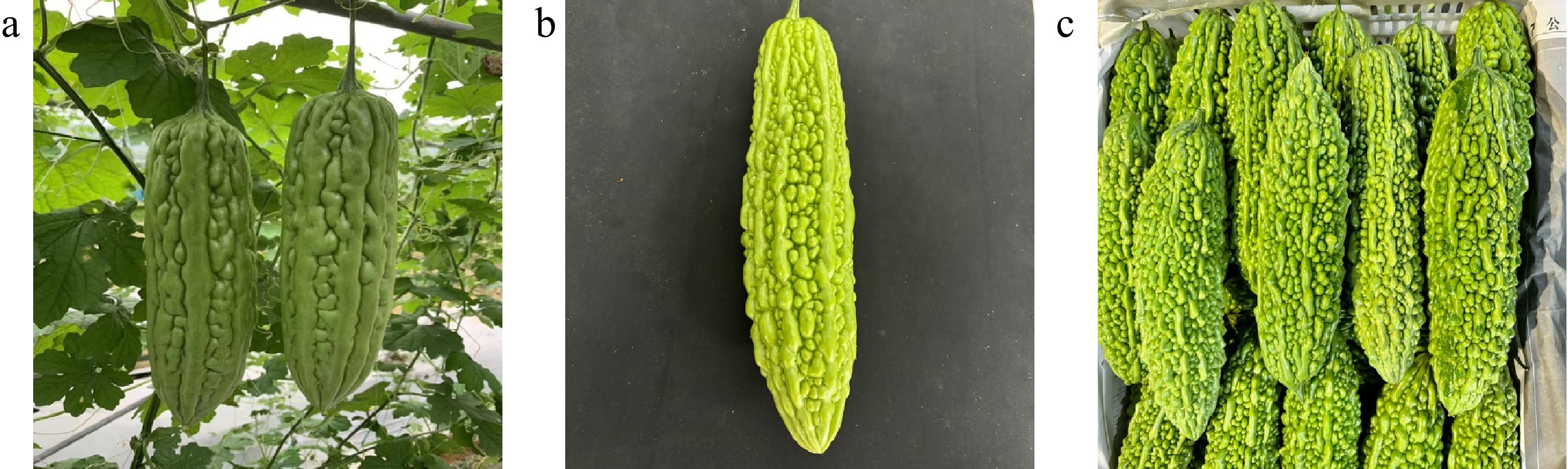
Figure 1.
Bitter gourd images captured in different acquisition scenarios. (a) Field scenes. (b) Indoor scenes. (c) Wholesale market scenes.
-
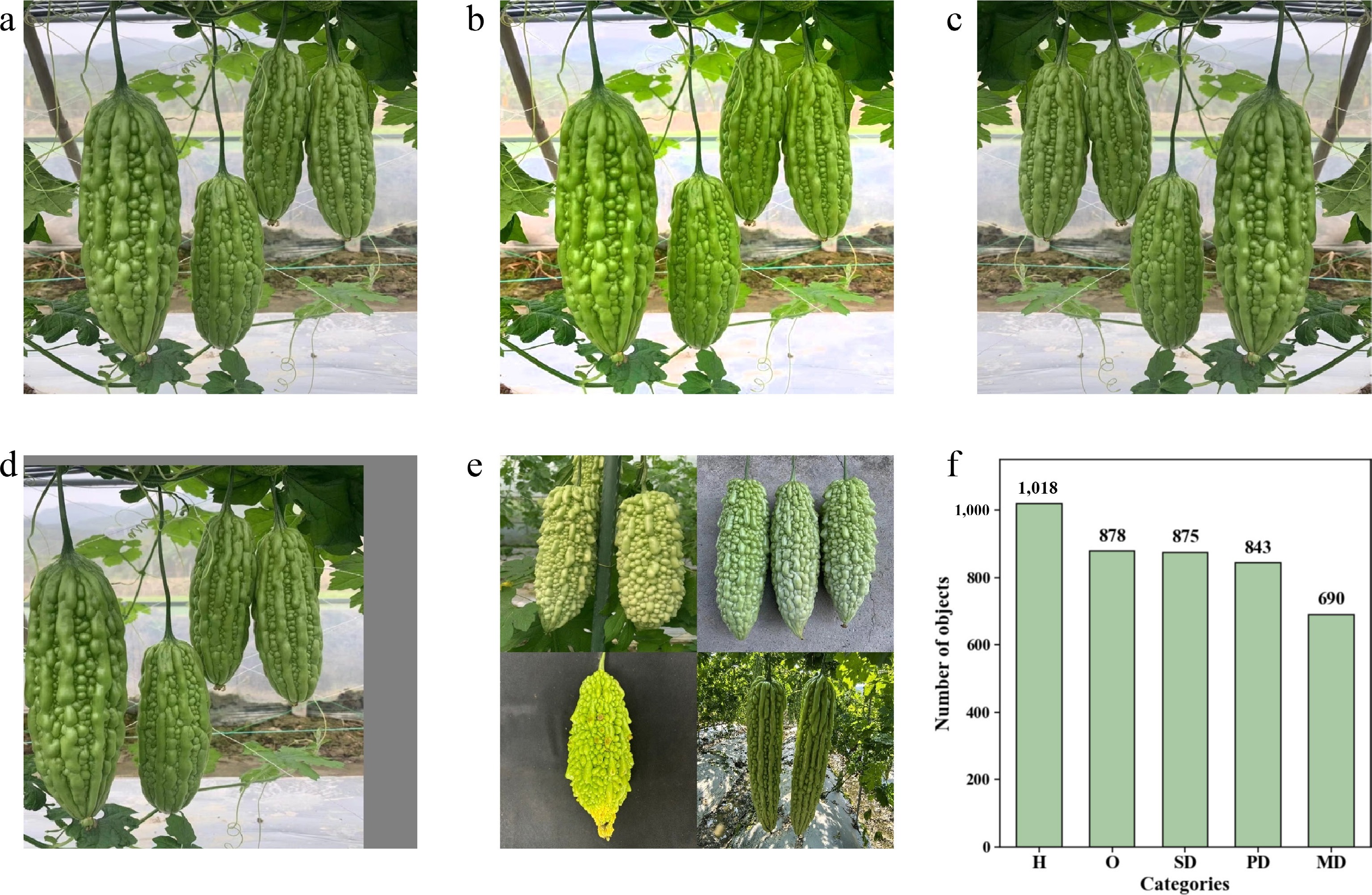
Figure 2.
Schematic diagram of data augmentation results and distribution of sample instances. (a) Original image. (b) Brightness adjustment. (c) Mirror flip. (d) Random translation. (e) Random combination. (f) Distribution of sample instances in the augmented dataset.
-
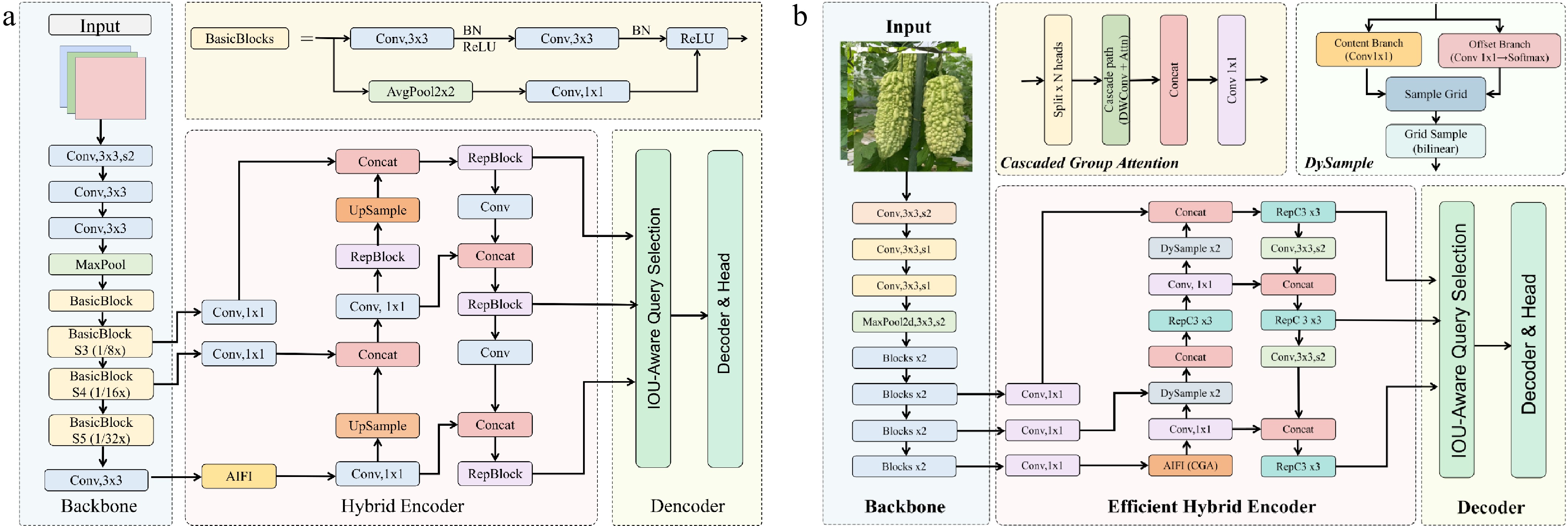
Figure 3.
Architecture comparison between the baseline and proposed models. (a) RTDETR-R18: the baseline network with ResNet-18 backbone, MHSA-based AIFI encoder, and GIoU loss. (b) CDS-RTDETR: the improved network integrating CGA in the AIFI module, DySample dynamic upsampler in the CCFM module, and Shape-IoU loss for bounding box regression.
-
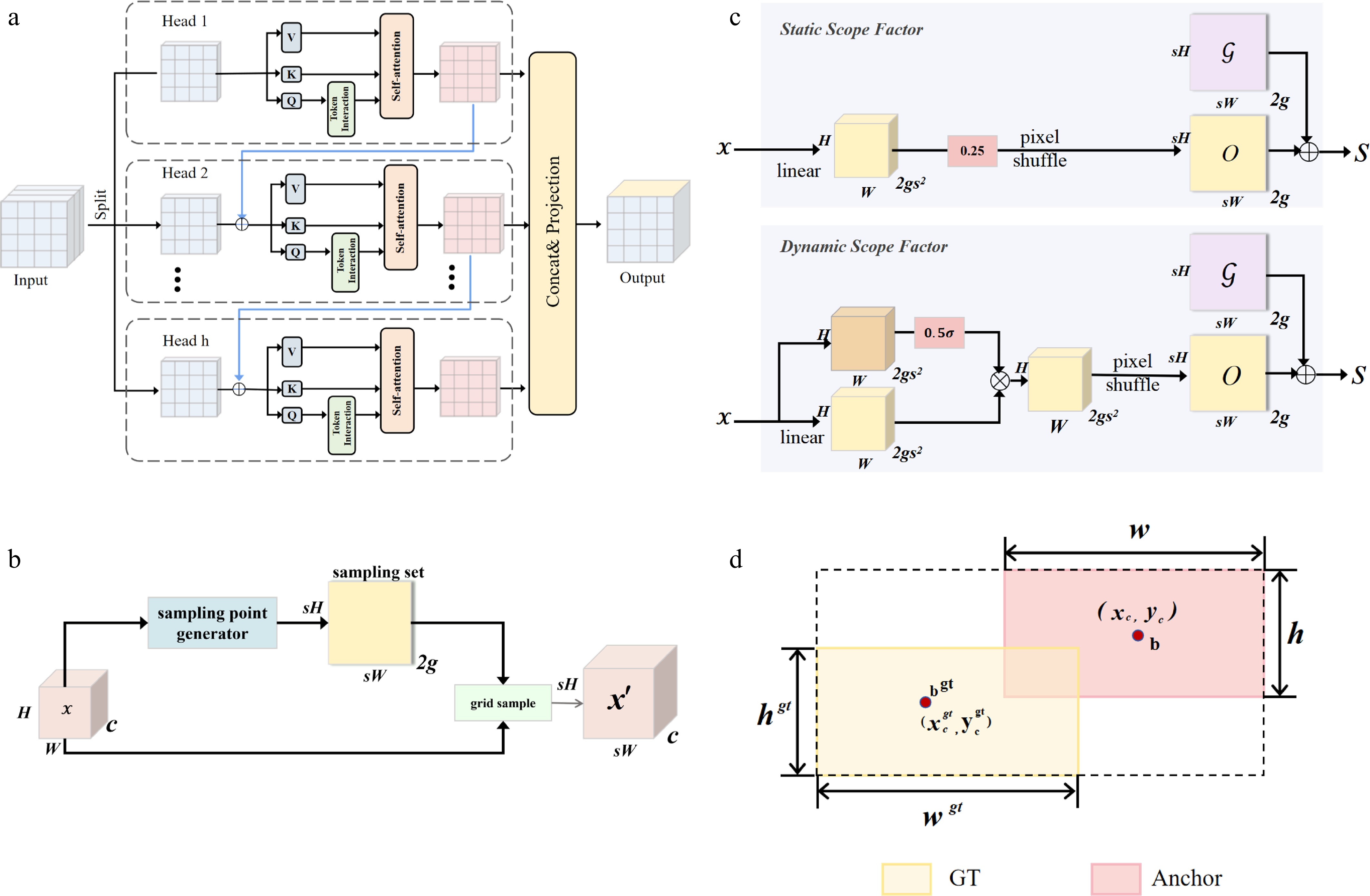
Figure 4.
Schematic diagrams of the key improvement modules in CDS-RTDETR. (a) Cascaded Group Attention (CGA). (b) Sampling-based dynamic upsampling in DySample. (c) Sampling point generator in DySample. (d) Shape-IoU loss function.
-
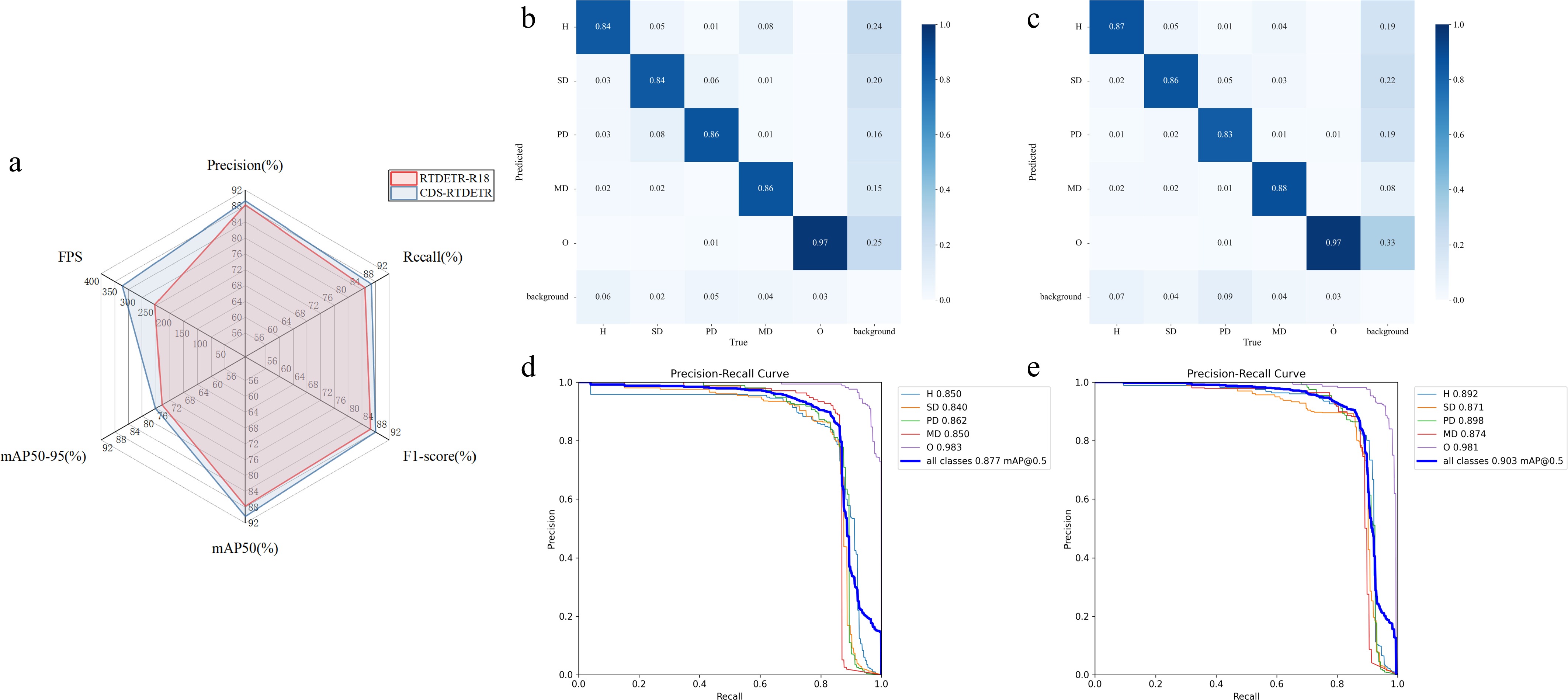
Figure 5.
Comprehensive performance evaluation of RTDETR-R18 and CDS-RTDETR. (a) Radar chart of model performance before and after improvement. (b) Normalized confusion matrix of RTDETR-R18. (c) Normalized confusion matrix of CDS-RTDETR. (d) Precision-Recall curves of RTDETR-R18. (e) Precision-Recall curves of CDS-RTDETR.
-
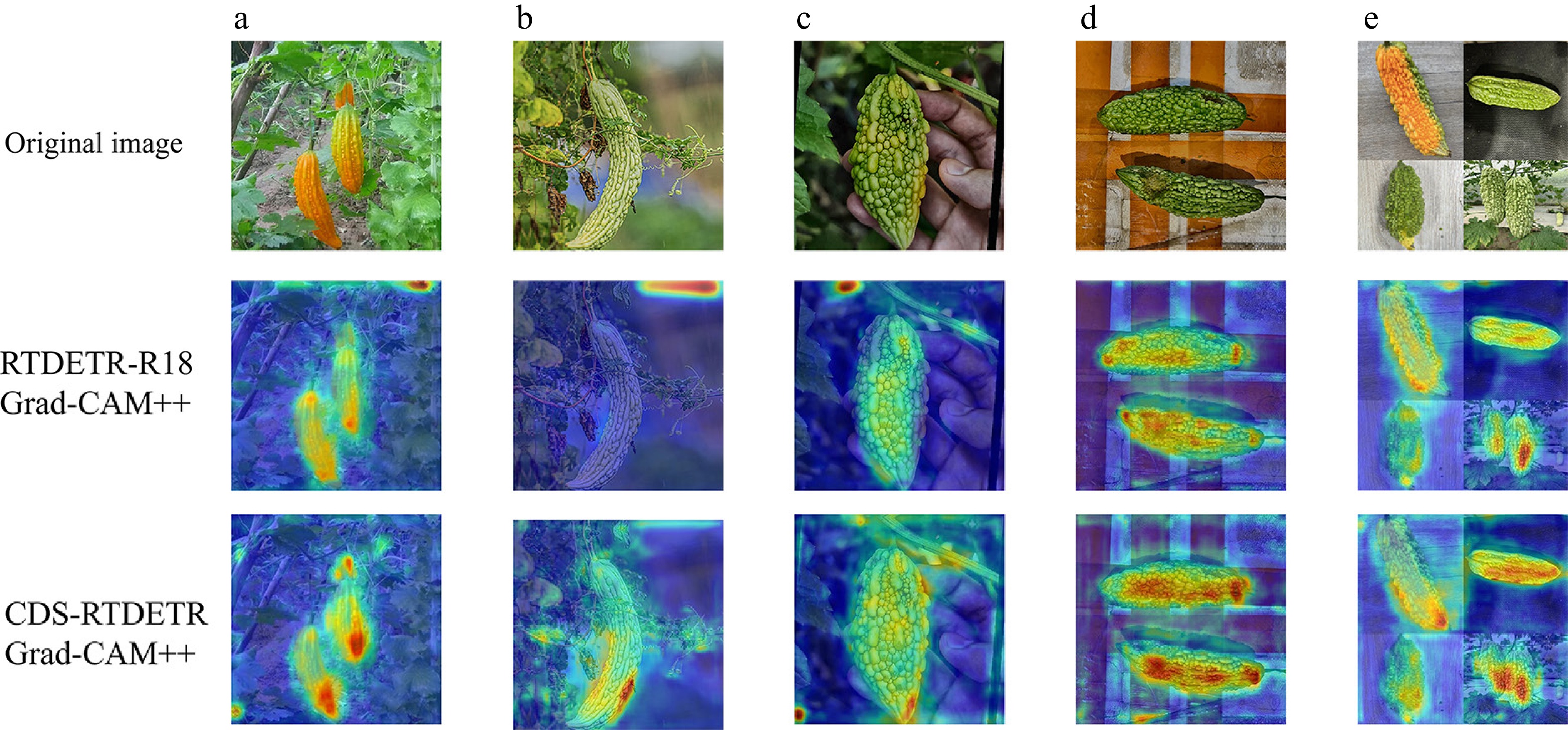
Figure 6.
Comparison of Grad-CAM++ heatmaps. (a)–(e) Five independent representative samples selected from the test set, with each column corresponding to a different bitter gourd image. The top row shows the original images, the middle row presents the activation maps generated by RTDETR-R18, and the bottom row presents the activation maps generated by CDS-RTDETR. The color scale ranges from blue (low attention) to yellow (medium attention) to red (high attention), representing the attention intensity of the models on defect-related regions. Warmer colors indicate stronger activation and more precise localization.
-
ID CGA DySample Shape-IoU GFLOPs Params
(M)Precision
(%)Recall
(%)F1-Score
(%)mAP50
(%)mAP75
(%)mAP50-95
(%)FPS Size
(MB)1 – – – 57.0 19.9 88.30 84.91 86.57 87.73 82.70 74.28 251.25 77.0 2 ✓ – – 57.0 19.7 88.57 85.79 87.16 89.02 83.22 74.73 362.32 76.4 3 – ✓ – 57.0 19.9 89.76 86.68 88.19 88.22 83.55 74.25 287.30 77.0 4 ✓ ✓ – 57.1 19.7 88.63 86.47 87.53 89.39 84.29 75.56 370.14 76.5 5 – – ✓ 57.0 19.9 88.27 87.96 88.12 89.48 83.14 75.09 264.18 77.0 6 ✓ – ✓ 57.0 19.7 90.62 83.97 87.17 89.31 84.19 74.76 359.96 76.4 7 – ✓ ✓ 57.0 19.9 88.92 87.10 88.00 88.29 84.02 74.68 299.77 77.0 8 ✓ ✓ ✓ 57.1 19.7 89.31 86.8 88.04 90.35 84.99 76.15 341.08 76.5 where '–' denotes that the original structure wasretained without modification, and '✓' indicates that the correspond-rhhzhyphening module was adopted. Table 1.
Results of ablation experiments.
-
ID Model Precision (%) Recall (%) F1-score (%) mAP50 (%) mAP75 (%) mAP50-95 (%) 1 CDS-RTDETR 89.31 86.80 88.04 90.35 84.99 76.15 2 RTDETR-R18 88.30 84.91 86.57 87.73 82.70 74.28 3 Hyper-YOLO 81.28 77.89 79.5 84.41 71.42 61.66 4 Mamba-YOLO 81.35 74.01 77.35 82.19 70.01 58.83 5 YOLOv5m 88.69 81.71 85.00 88.82 82.34 69.04 6 YOLOv8m 86.89 81.59 84.08 89.12 81.17 69.93 7 YOLOv10m 67.45 57.63 61.77 67.33 57.82 49.71 8 YOLOv11m 82.93 80.92 81.87 87.98 78.28 67.00 9 YOLOv12m 88.66 81.98 85.08 90.04 82.12 70.49 10 YOLOv13s 82.20 74.94 78.09 83.23 72.38 62.42 11 YOLOv26m 75.27 68.75 71.80 77.14 69.27 58.80 All models were trained onthe same dataset and under identical training configurations. Table 2.
Comparative experimental results.
Figures
(6)
Tables
(2)