-
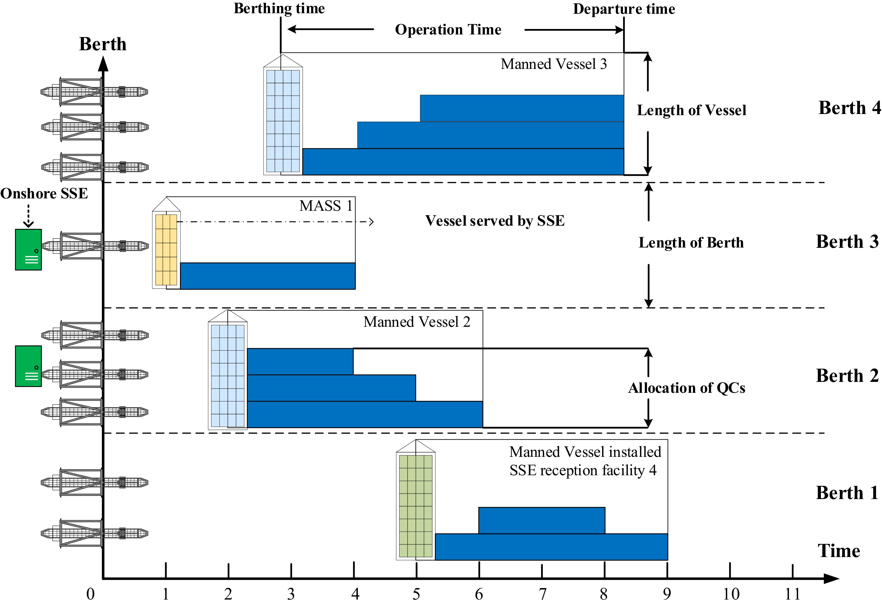
Figure 1.
Space-time diagram of BACAP with SSE allocation.
-
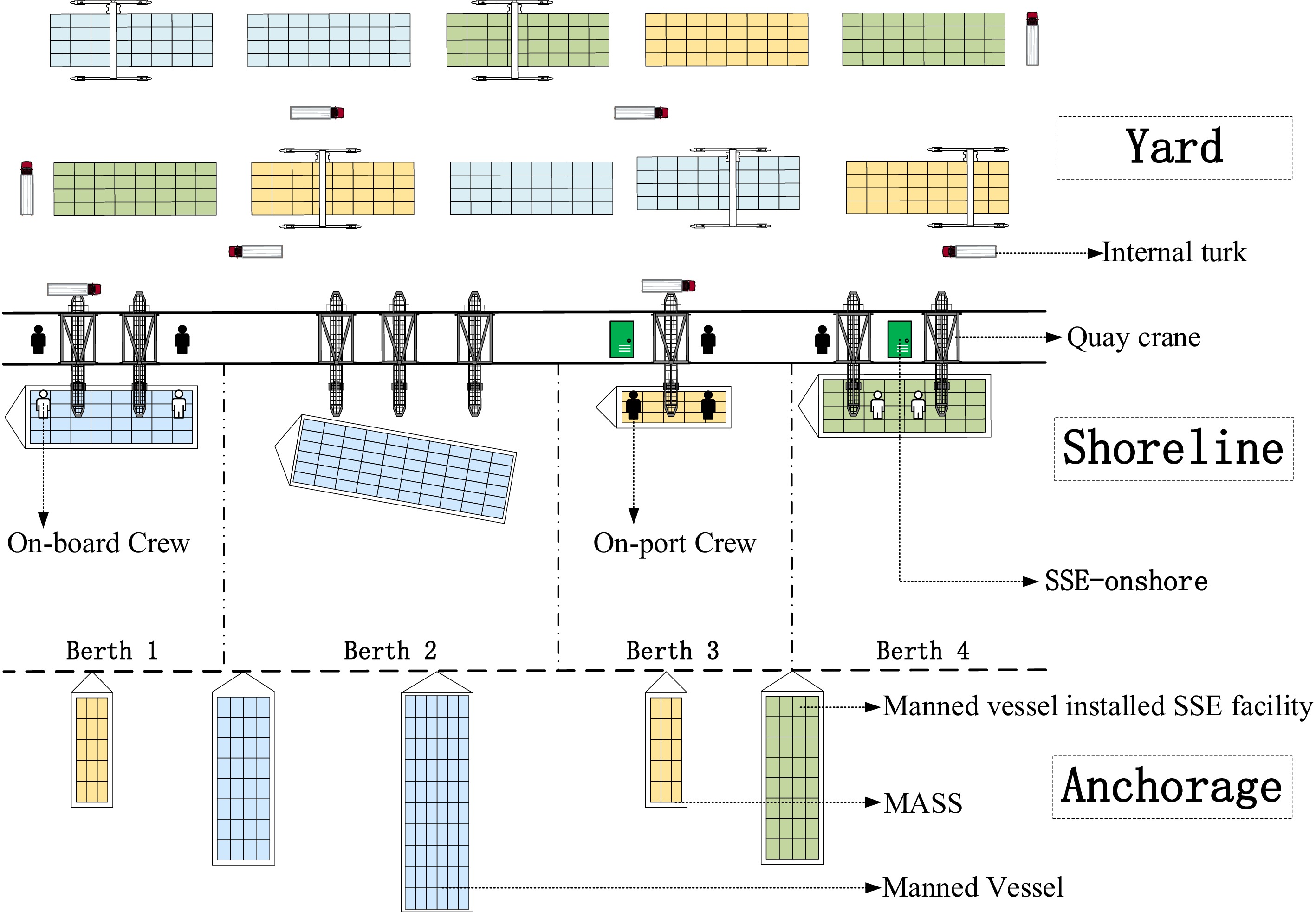
Figure 2.
Shore operations of MASS and manned vessels.
-
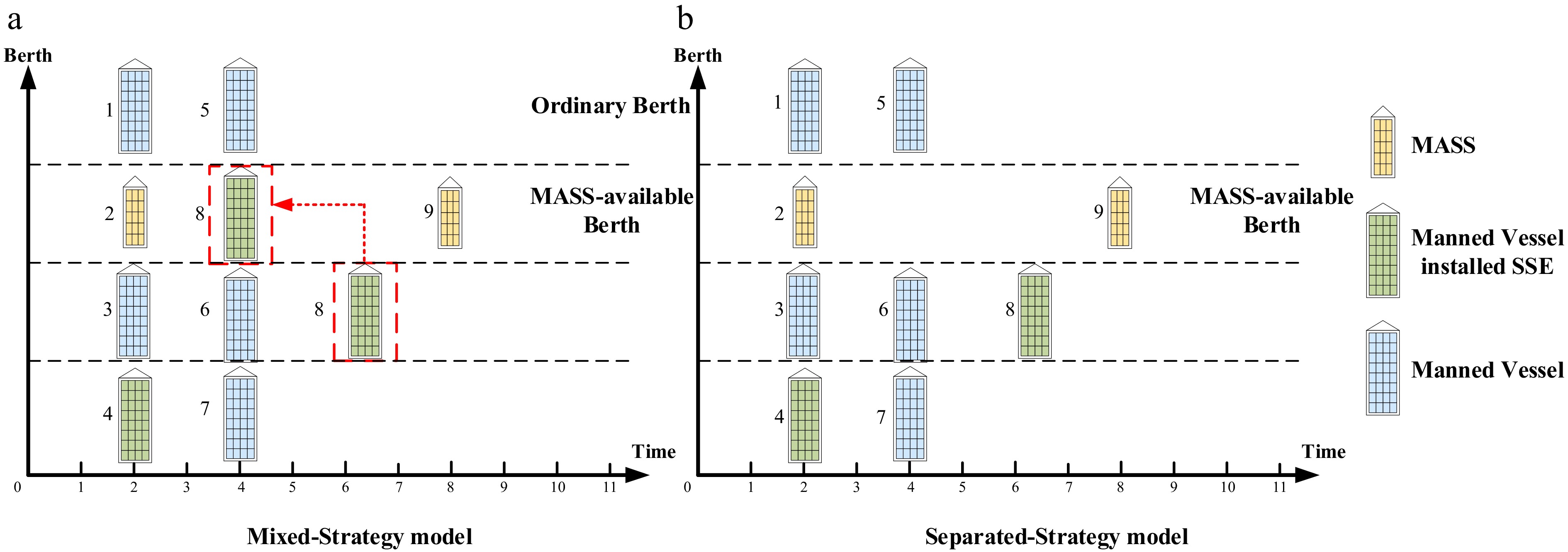
Figure 3.
Berth allocation model for Mixed-Strategy and Separated-Strategy.
-
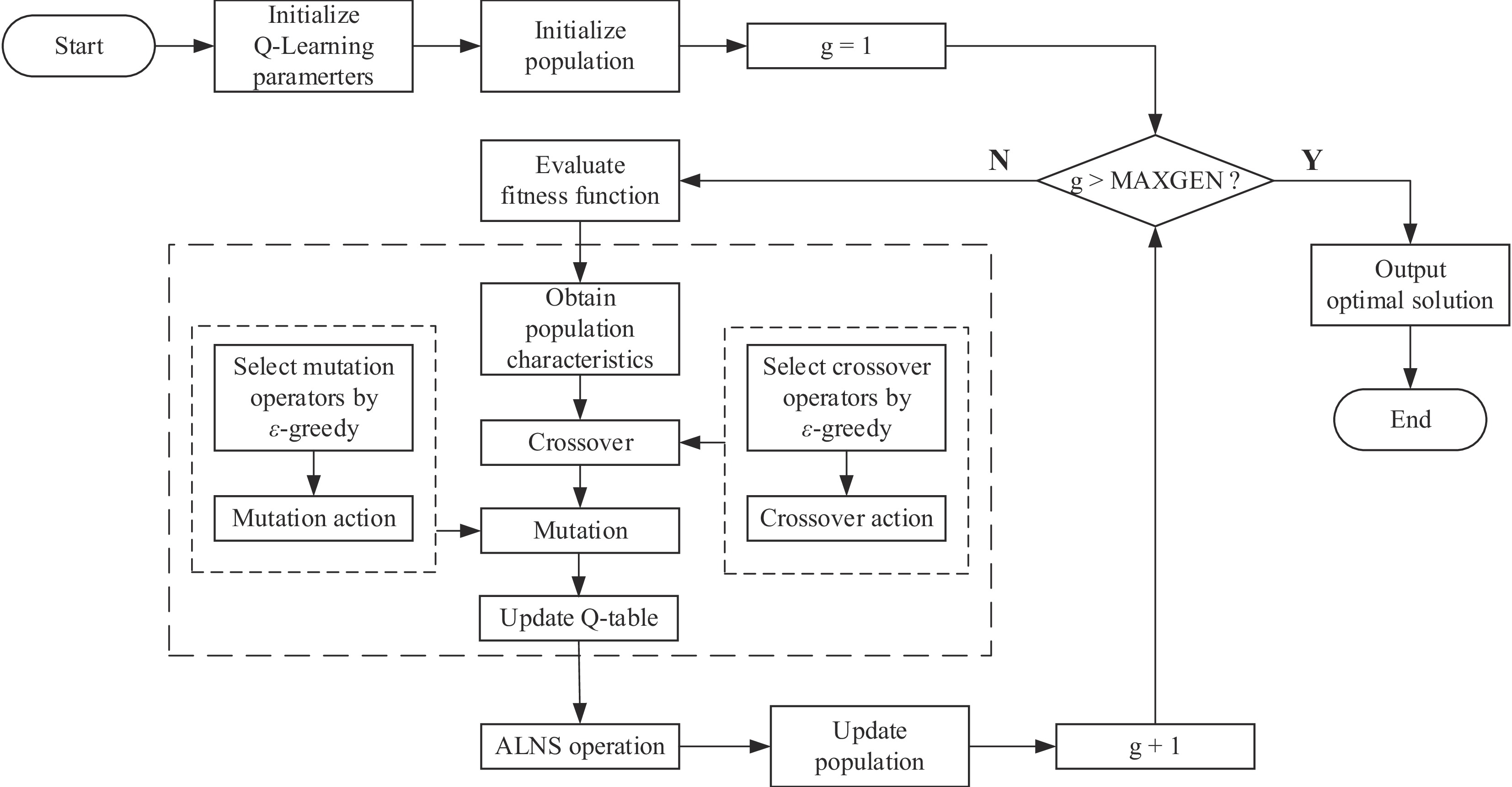
Figure 4.
The flowchart of the GA + ALNS algorithm combined with Q-learning.
-
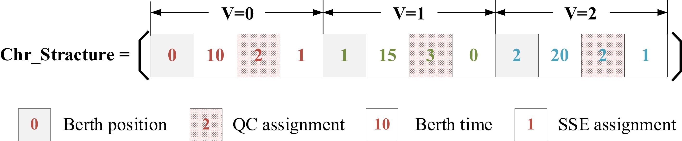
Figure 5.
The example of chromosome structure.
-
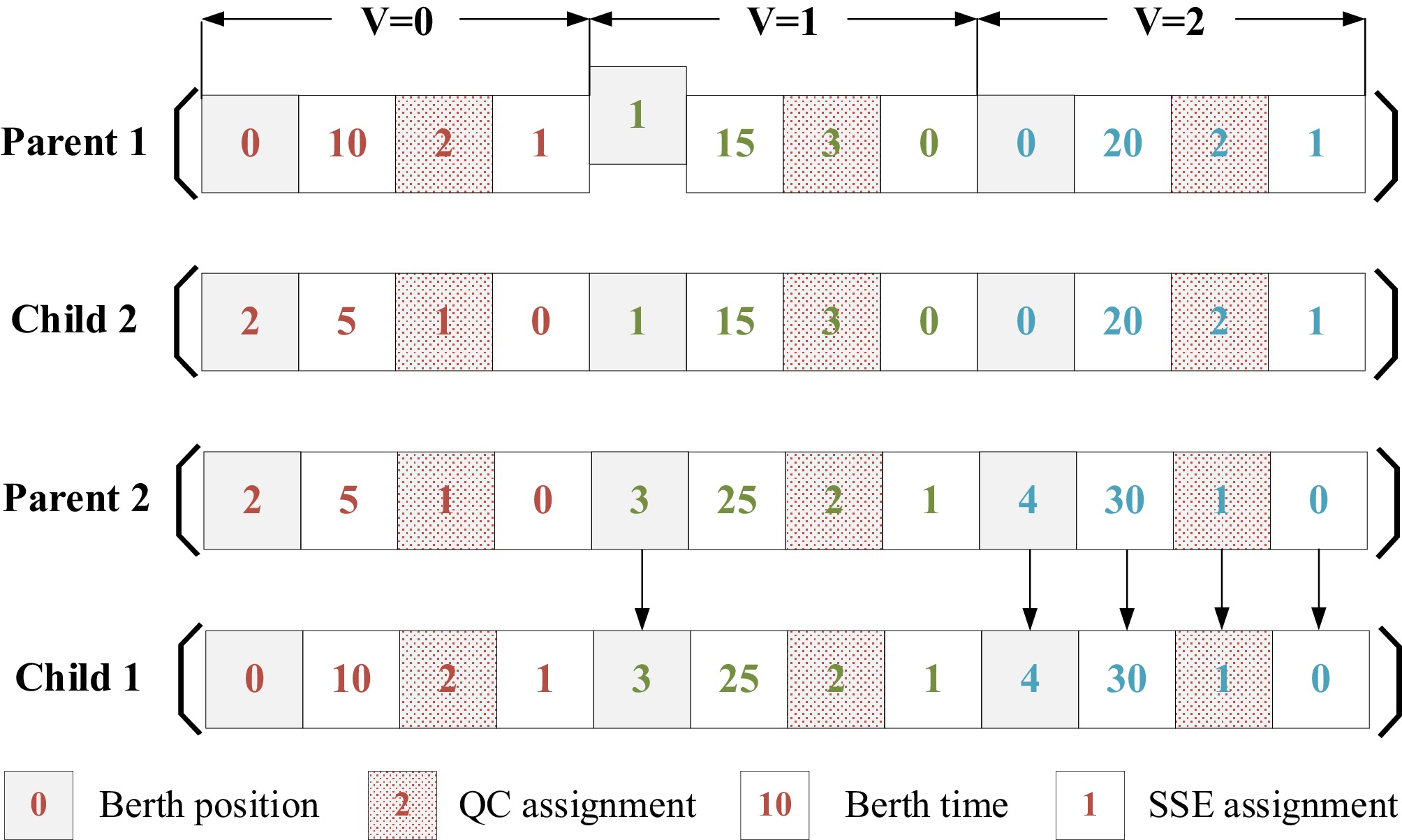
Figure 6.
Single-point crossover.
-
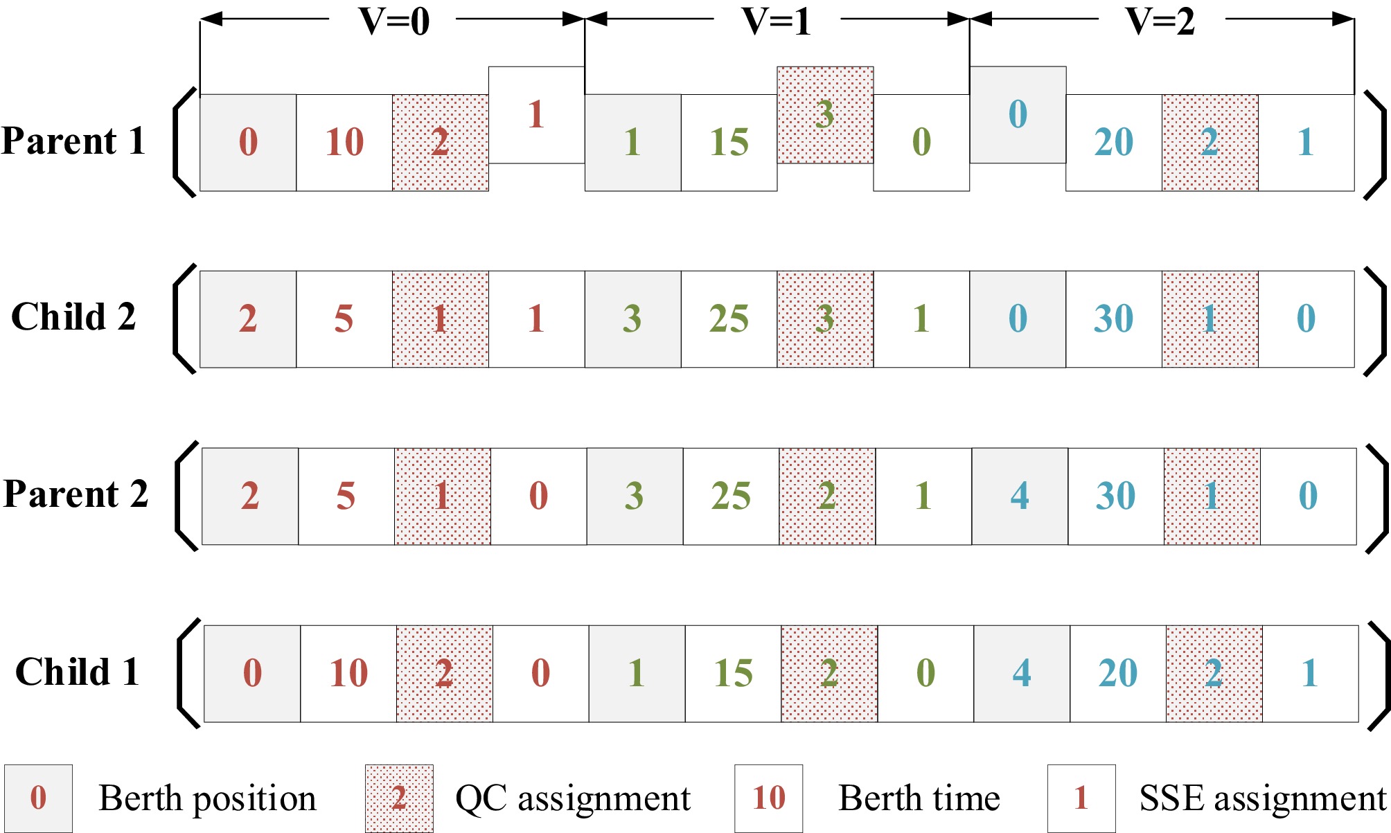
Figure 7.
Multi-point crossover.
-
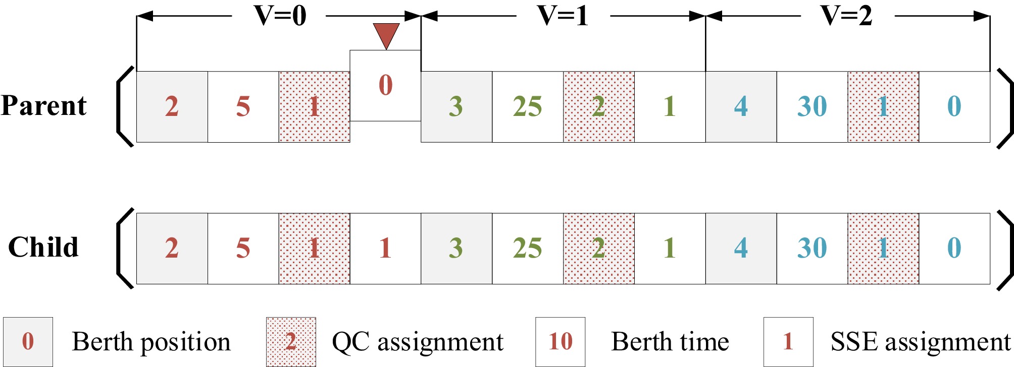
Figure 8.
Endpoint mutation.
-
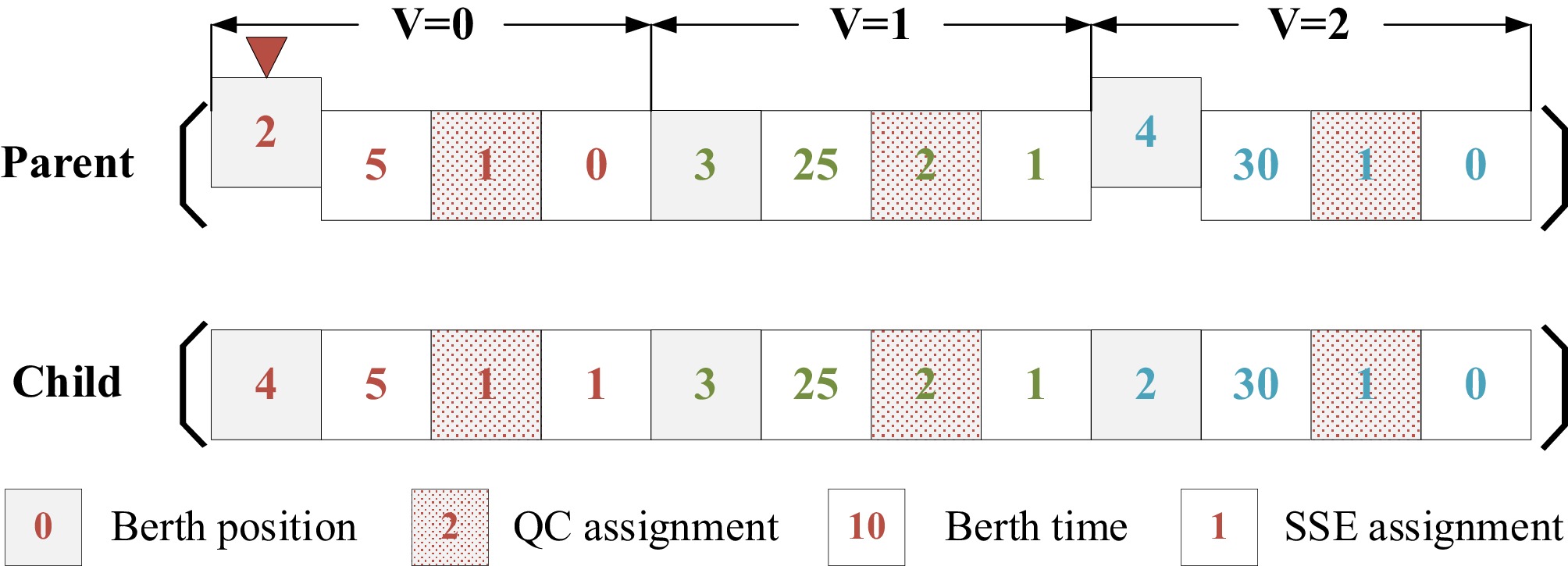
Figure 9.
Two-point mutation.
-
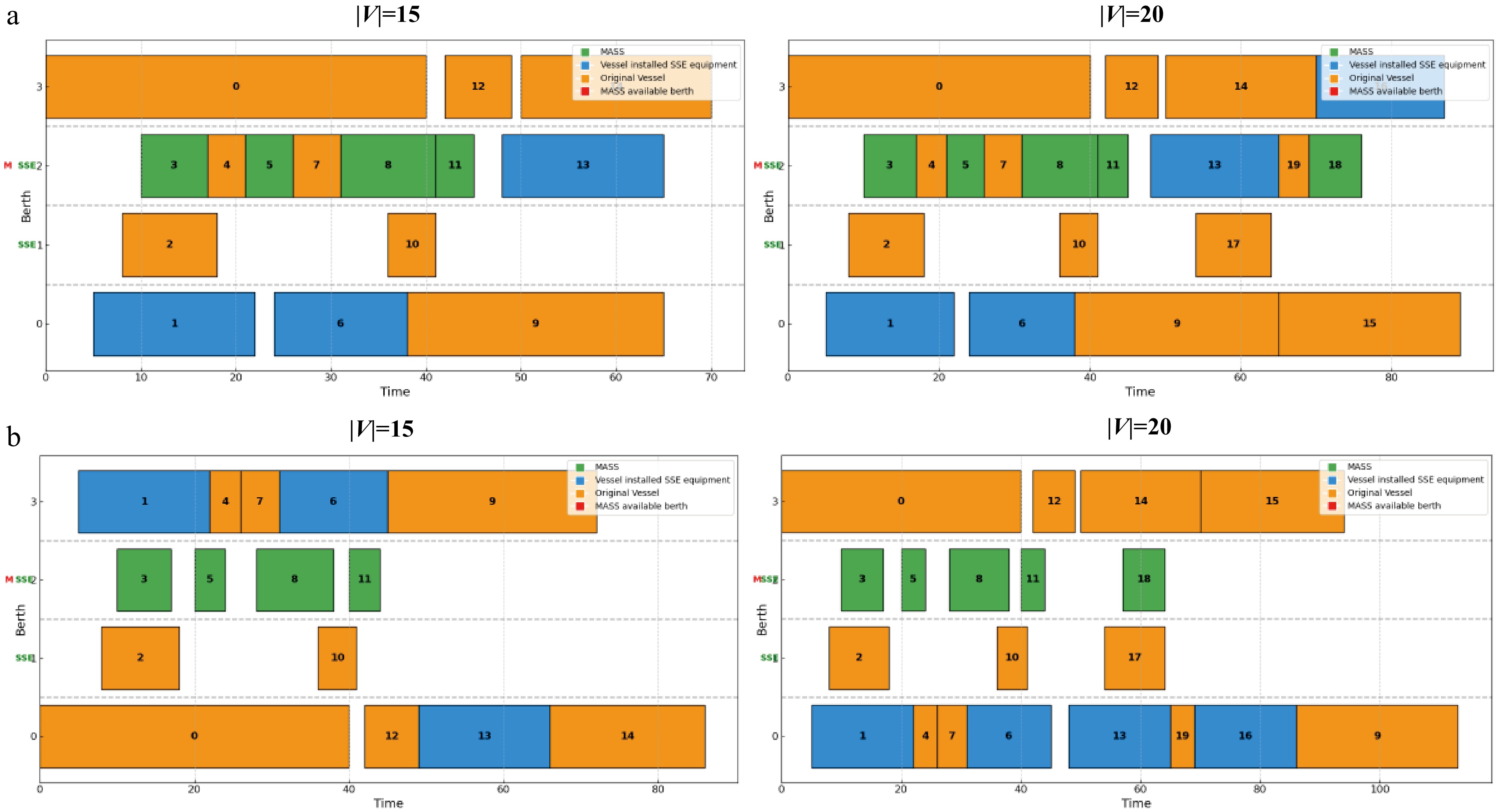
Figure 10.
Space-time diagram of (a) Mixed-Strategy and (b) Separated-Strategy.
-
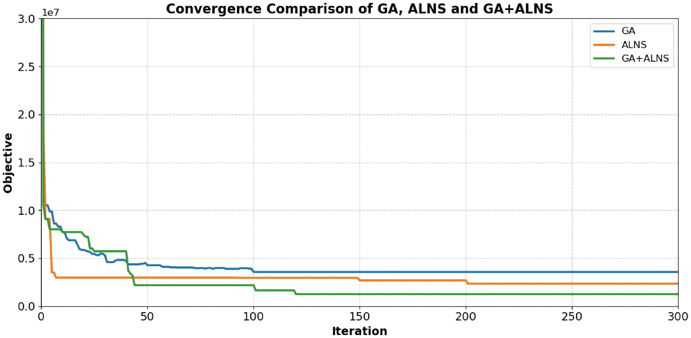
Figure 11.
Convergence comparison of algorithms.
-
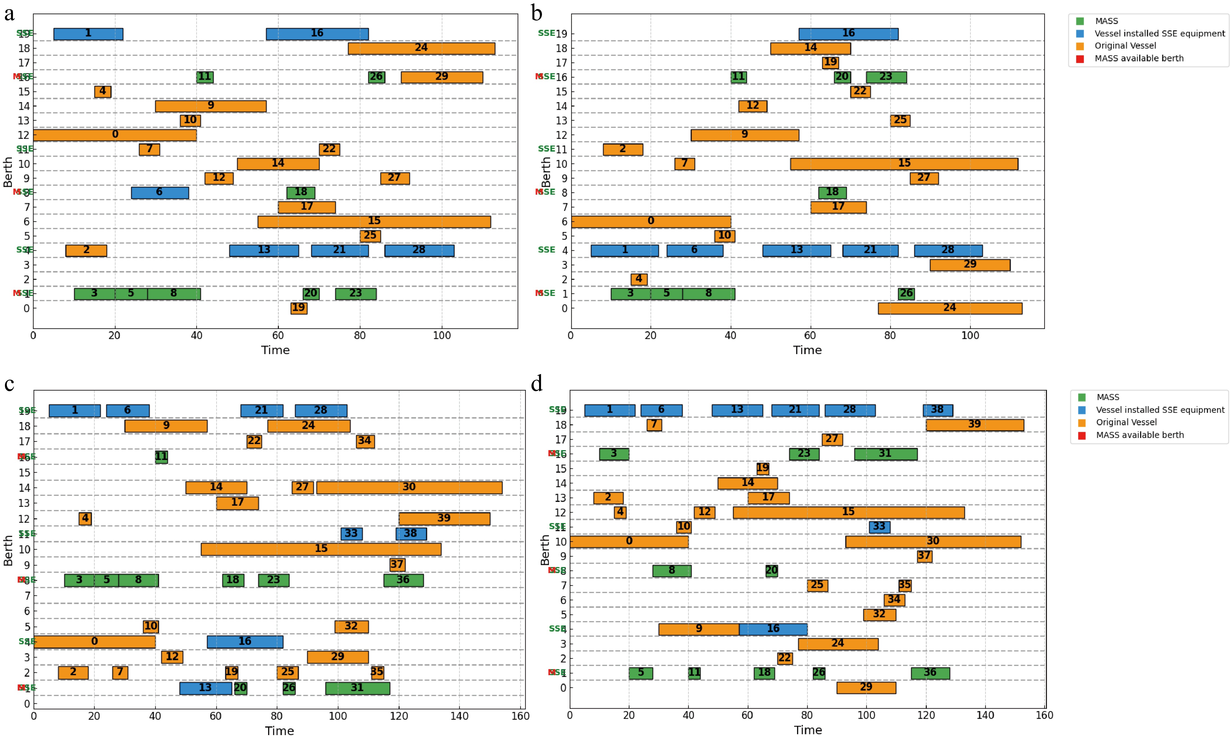
Figure 12.
Berth allocation schemes at YICT under Mixed-Strategy and Separated-Strategy. (a)
$ \left| V\right| $ $ \left| V\right| $ $ \left| V\right| $ $ \left| V\right| $ -
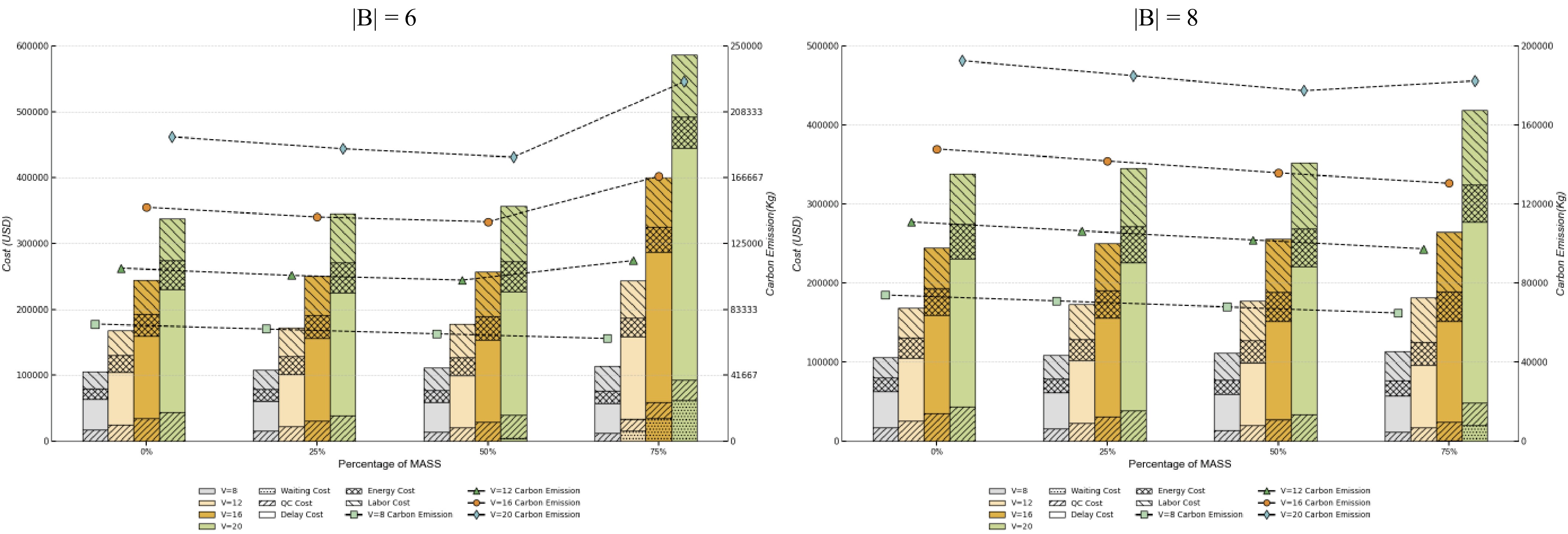
Figure 13.
The impact of MASS quantity on cost composition and carbon emissions.
-
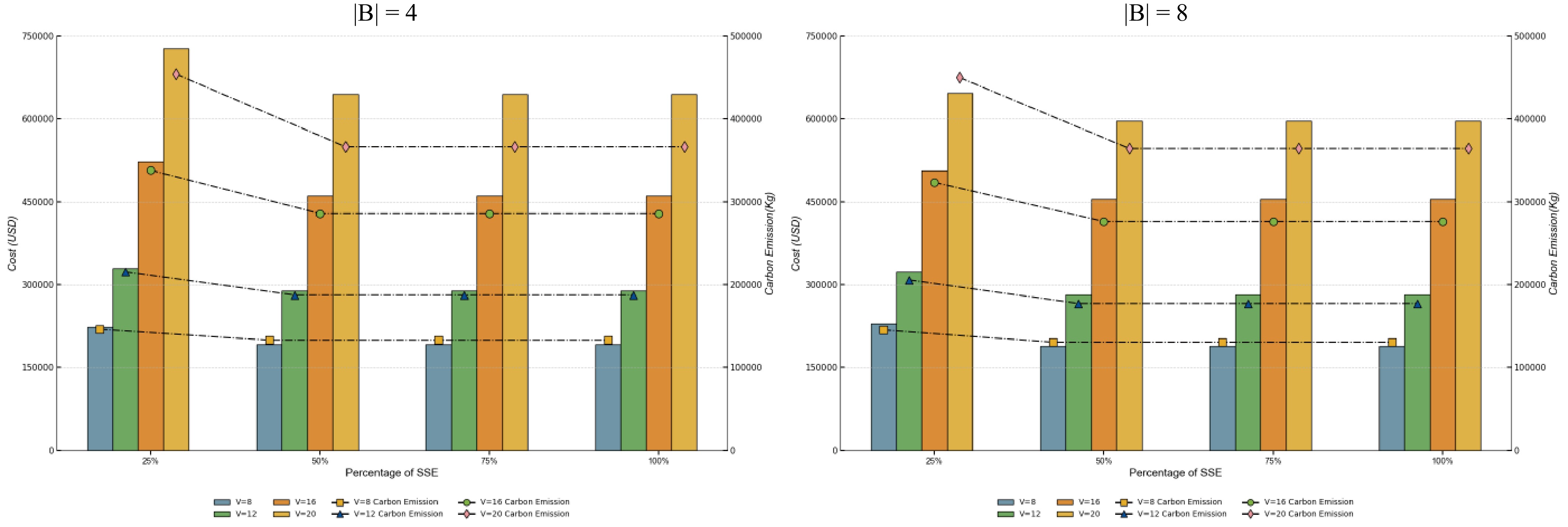
Figure 14.
The impact of the change in the quantity of SSE on total cost and carbon emissions.
-
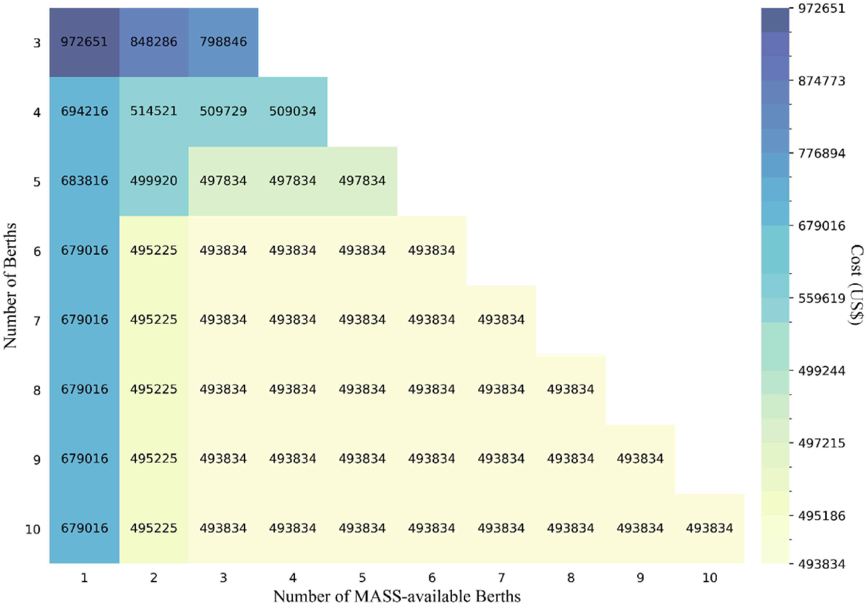
Figure 15.
The impact of the change in the quantity of MASS-available berths on total cost.
-
Paper BAP QCAP SSE Method Vessel type Zhang & Wang[13] √ Solver MASS Zhen et al.[15] √ √ CG Manned vessel Tang et al.[11] √ √ LNS Manned vessel Yu et al.[16] √ √ √ N-NSGA-II Manned vessel Guo et al.[12] √ √ ALNS Manned vessel Wang et al.[17] √ √ √ AICSA Manned vessel Martin-Iradi et al.[23] √ ALNS Manned vessel Yue et al.[18] √ √ NSGA-III Manned vessel Shen et al.[14] √ SA Manned vessel + MASS This study √ √ √ GA + ALNS Manned vessel + MASS Table 1.
Literature review.
-
Vessel types Sailing Anchoring Berthing Diesel-powered vessels with SSE MEa fuel AEb fuel AE fuel/SSE Diesel-powered vessels without SSE ME fuel AE fuel AE fuel Hybrid-powered MASS ME fuel Stored electricity SSE Electric-powered MASS Stored electricity Stored electricity SSE a Main engine. b Auxiliary engines. Table 2.
The type of energy consumed by different types of ships at different periods[26].
-
Notation Explanation Sets $ V $ The set of vessels, $ V=\left\{1,\;2,\;3,\;\cdots ,\;\left| V\right| \right\} $ $ \left| V\right| $ $ i\in V $ $ B $ The set of berths, $ B=\left\{1,2,3,\cdots ,\left| B\right| \right\} $ $ \left| B\right| $ $ b\in B $ $ Q $ The set of QCs, $ Q=\left\{1,2,3,\cdots ,\left| Q\right| \right\} $ $ \left| Q\right| $ $ q\in Q $ $ T $ The set of time units, $ T=\left\{1,2,3,\cdots \left| T\right| \right\} $ $ \left| T\right| $ $ t\in T $ Parameters $ {C}_{1} $ Unit cost of waiting berth at anchorage $ {C}_{2} $ Unit cost of using the quay cranes $ {C}_{3} $ The SSE unit price $ {C}_{4} $ The fuel oil unit price $ {C}_{5} $ Unit cost of delay penalty $ {C}_{6} $ Labor cost per unit time $ \lambda $ Reward factor of using SSE service during berthing $ {L}_{i} $ Length of vessel $ i $ $ {L}_{b} $ Length of berth $ b $ $ {A}_{i} $ Arrival time of vessel $ i $ $ {K}_{i} $ Number of loading or unloading containers of vessel $ i $ $ {D}_{i} $ The expected departure time of vessel $ i $ $ q_{\mathrm{i}}^{\min } $ Minimum number of quay cranes assigned to vessel $ i $ $ q_{i}^{\max } $ Maximum number of quay cranes assigned to vessel $ i $ $ \eta $ Speed of quay cranes $ {E}_{i} $ Auxiliary engine power of vessel $ i $ $ {N}^{s} $ The total number of terminal stevedores $ {N}^{c} $ The total number of terminal tally clerks $ Crew_{s}^{mass} $ The number of stevedores in each crew assigned to MASS $ Crew_{c}^{mass} $ The number of tally clerks in each crew assigned to MASS $ Crew_{s}^{m} $ The number of stevedores in each crew assigned to manned vessel $ Crew_{c}^{m} $ The number of tally clerks in each crew assigned to manned vessel $ M $ A large positive number Auxiliary variables $ Eq{v}_{i} $ Binary, 1 if vessel $ i $ $ Eq{v}_{b} $ Binary, 1 if berth $ b $ $ M{A}_{i} $ Binary, 1 if vessel $ i $ $ B_{b}^{mass} $ Binary, 1 if berth $ b $ Decision variables $ {S}_{i} $ Berthing time of vessel $ i $ $ {P}_{i} $ Berth allocated to vessel $ i $ $ {d}_{i} $ Departure time of vessel $ i $ $ W_{itq}^{s} $ Integer, allocate the number of stevedores of
quay crane$ q $ $ i $ $ t $ $ W_{itq}^{c} $ Integer, allocate the number of tally clerks of
quay crane$ q $ $ i $ $ t $ $ {O}_{i} $ Binary, 1 if vessel $ i $ $ {X}_{itb} $ Binary, 1 if vessel $ i $ $ b $ $ t $ $ {Y}_{itq} $ Binary, 1 if quay crane $ q $ $ i $ $ t $ $ {Z}_{ijb} $ Binary, 1 if vessel $ i $ $ j $ $ b $ $ j $ $ i $ Table 3.
Notations of the model.
-
Score Criteria description 3 Find a better solution or equal to the optimal solution after using the ALNS operators 1.5 Find a better solution or equal to the current solution after using the ALNS operators 0 Find a solution that is worse than the current solution after using the ALNS operators Table 4.
The score of destroyed and repaired operators.
-
Parameters Value Ref. $ {C}_{1} $ 800 US ${\$} $ Wang et al.[34] $ {C}_{2} $ 240 US ${\$} $ Model assumption $ {C}_{3} $ 0.15918 US ${\$} $ Peng et al.[33] $ {C}_{4} $ 0.13382 US ${\$} $ Peng et al.[33] $ {C}_{5} $ 2400 US ${\$} $ Wang et al.[34] $ {C}_{6} $ 40 US ${\$} $ Model assumption $ \eta $ 30 TEU/h Model assumption $ \lambda $ 0.4 HPA[30] $ M $ 100,000 Model assumption $ {c}^{e} $ 0.54 kg/kWh Hall[35] $ {c}^{f} $ 0.6412 kg/kWh Hall[35] Table 5.
Values of some parameters.
-
$ \left| V\right| $ $ \left| B\right| $ $ \left| Q\right| $ $ \left| B_{b}^{mass}\right| $ Gurobi solving results GAP (%) Mixed-Strategy Separated-Strategy $ Ob{j}_{1} $ ${\$} $ Times (s) $ Ob{j}_{2} $ ${\$} $ Times (s) 6 4 9 1 154,678.04 1.76 158,881.69 1.70 2.65 6 12 2 151,661.30 0.94 152,258.62 0.60 0.39 8 15 3 151,661.30 0.96 151,661.30 0.91 0.00 10 18 4 151,661.30 1.14 151,661.30 1.02 0.00 8 4 9 1 192,980.09 2.58 222,112.94 2.23 13.12 6 12 2 189,577.96 2.19 190,560.66 0.92 0.52 8 15 3 189,577.96 1.98 189,577.96 1.54 0.00 10 18 4 189,577.96 2.41 189,577.96 2.15 0.00 10 4 9 1 308,054.41 54.73 334,629.59 3.35 7.94 6 12 2 269,410.28 2.08 296,034.98 2.00 8.99 8 15 3 269,410.28 3.31 295,052.28 2.46 8.69 10 18 4 269,410.28 2.93 269,410.28 2.68 0.00 15 4 9 1 435,356.64 60.47 537,437.17 10.52 18.99 6 12 2 398,567.20 29.29 400,147.21 3.94 0.39 8 15 3 398,567.20 30.48 398,567.20 7.91 0.00 10 18 4 398,567.20 9.87 398,567.20 8.89 0.00 20 4 9 1 727,758.10 1,641.2 889,589.73 627.49 18.19 6 12 2 − 3,600 − 3,600 − 8 15 3 − 3,600 − 3,600 − 10 18 4 − 3,600 − 3,600 − Average 285,086.91 307,395.8 7.26 Table 6.
Gurobi solution results.
-
Cost (US ${\$} $ $ \left| V\right| $ 8 10 15 20 Average GAP (%) Total cost Mixed 192,980.09 308,054.41 435,356.64 727,758.1 363,765.46 15.1 Separated 222,112.94 334,629.59 537,437.17 889,589.73 428,530.22 Waiting cost Mixed 2,400 11,200 12,000 50,400 15,680 51.2 Separated 11,200 19,200 36,800 88,000 32,160 QCs cost Mixed 23,184 31,104 41,808 56,016 34,147.2 18.8 Separated 23,184 31,104 43,440 57,648 34,800 Energy cost Mixed 29,676.09 42,190.41 58,628.64 87,582.1 48,338.26 13.9 Separated 33,208.94 46,365.59 69,477.17 106,981.73 56,130.22 Delay cost Mixed 120,000 103,200 175,200 256,800 446,400 15.8 Separated 141,600 120,000 189,600 321,600 549,600 Table 7.
Key costs calculated under Mixed-Strategy and Separated-Strategy.
-
$ \left| V\right| $ Carbon emissions (kg) GAP (%) Mixed-Strategy Separated-Strategy 6 111,899.76 116,708.76 4.12 8 140,946.12 157,873.8 10.72 10 200,422.92 219,132.36 8.54 15 269,819.52 329,159.04 18.03 20 412,487.16 507,615.36 18.74 Average 227,115.1 26,6097.9 14.65 Table 8.
Comparison of carbon emissions between tow berth allocation strategies.
-
Algorithm Our method ALNS GA $ \left| V\right| $ Case $ Ob{j}_{1} $ CT (s) Gap $ Ob{j}_{2} $ CT (s) Gap $ Ob{j}_{3} $ CT (s) Gap 6 1 156,378.04 5.55 1.09 157,044.07 5.81 1.51 158,442.37 1.85 2.38 2 152,876.58 5.63 0.79 153,481.17 7.88 1.19 154,641.17 2.00 1.93 3 152,229.14 5.65 0.37 153,043.34 10.61 0.90 154,297.42 1.92 1.71 4 151,917.81 6.38 0.17 153,312.35 7.75 1.08 154,205.57 1.97 1.65 8 1 195,932.36 6.71 1.51 198,024.80 7.45 2.55 203,866.44 2.37 5.34 2 192,382.78 6.87 1.46 195,104.03 8.63 2.83 207,339.07 1.85 8.57 3 191,648.06 6.86 1.08 194,461.90 11.24 2.51 202,450.95 2.42 6.36 4 191,184.36 6.78 0.84 193,666.21 15.72 2.11 201,704.02 2.52 6.01 10 1 316,972.67 7.67 2.81 334,296.79 12.38 7.85 350,287.69 3.04 12.06 2 276,229.36 7.80 2.47 291,651.20 14.48 7.63 306,379.28 2.84 12.07 3 275,324.49 7.91 2.15 285,127.84 18.96 5.51 301,053.86 3.02 10.51 4 275,012.08 8.70 2.04 281,047.88 21.74 4.14 298,938.24 3.84 9.88 15 1 453,425.37 11.45 3.98 469,563.09 21.57 7.28 493,484.25 4.29 11.78 2 414,993.68 11.29 3.96 428,555.32 25.07 7.00 452,447.37 4.51 11.91 3 416,609.86 10.73 4.33 425,594.14 31.25 6.35 442,073.82 4.43 9.84 4 414,493.16 11.80 3.84 422,031.97 30.39 5.56 442,394.65 4.02 9.91 20 1 771,630.94 17.76 5.69 801,368.39 30.28 9.19 881,017.78 5.98 17.40 2 651,233.08 20.77 − 697,908.48 41.27 − 727,124.39 6.01 − 3 629,316.41 22.37 − 652,647.68 54.01 − 672,714.46 5.95 − 4 627,808.35 25.65 − 644,477.01 49.39 − 661,304.62 5.69 − 30 1 1,044,593.77 29.68 − 1,377,603.23 68.11 − 1,667,353.24 9.43 − 2 932,048.17 36.26 − 999,053.32 86.65 − 1,345,368.42 9.03 − 3 921,896.12 37.47 − 968,950.33 106.33 − 1,120,027.34 8.75 − 4 917,101.77 41.94 − 963,263.93 100.25 − 1,114,765.17 8.96 − 40 1 1,574,540.08 54.04 − 1,701,024.87 155.63 − 2,340,866.86 18.76 − 2 1,341,607.22 66.72 − 1,588,796.82 161.82 − 2,063,518.60 19.35 − 3 1,189,445.17 68.39 − 1,562,007.22 165.73 − 1,808,089.58 18.85 − 4 1,060,306.03 70.96 − 1,300,407.35 209.49 − 1,512,966.78 23.36 − Average 567,469.18 22.13 2.27 628,339.81 52.85 4.42 729,968.69 6.68 8.19 Table 9.
Comparison of results of different algorithms.
-
Parameters Value Total number of berths 20 Total number of QCs 85 Total number of MASS-available berths 3 Total number of SSE facilities 6 The planning horizon 168 Total number of vessels 30, 40 Total number of MASSs 8, 10 Total number of manned vessels equipped
with SSE reception facilities6, 8 Table 10.
Parameter settings based on the real environment of YICT.
-
$ \left| V\right| $ Strategies Novel GA + ALNS GA + ALNS ALNS GA $ Ob{j}_{1} $ CT (s) $ Ob{j}_{2} $ CT (s) $ Ob{j}_{3} $ CT (s) $ Ob{j}_{4} $ CT (s) 30 Mixed 876,010.54 48.3 917,101.77 46.2 933,979.66 77.4 935,903.24 34.5 Separated 876,281.38 50.5 917,310.26 54.4 935,664.19 85.1 936,230.78 40.3 40 Mixed 1,187,623.68 62.8 1,223,508.41 64.9 1,305,649.48 94.3 1,317,627.52 56.7 Separated 1,218,904.03 65.2 1,292,038.28 70.6 1,334,883.52 98.7 1,352,913.46 60.4 Average 1,039,704.91 56.7 1,087,489.68 59.03 1,127,544.21 88.87 1,135,668.75 47.98 Table 11.
Results of different algorithms at YICT under Mixed-Strategy and Separated-Strategy.
Figures
(15)
Tables
(11)