-
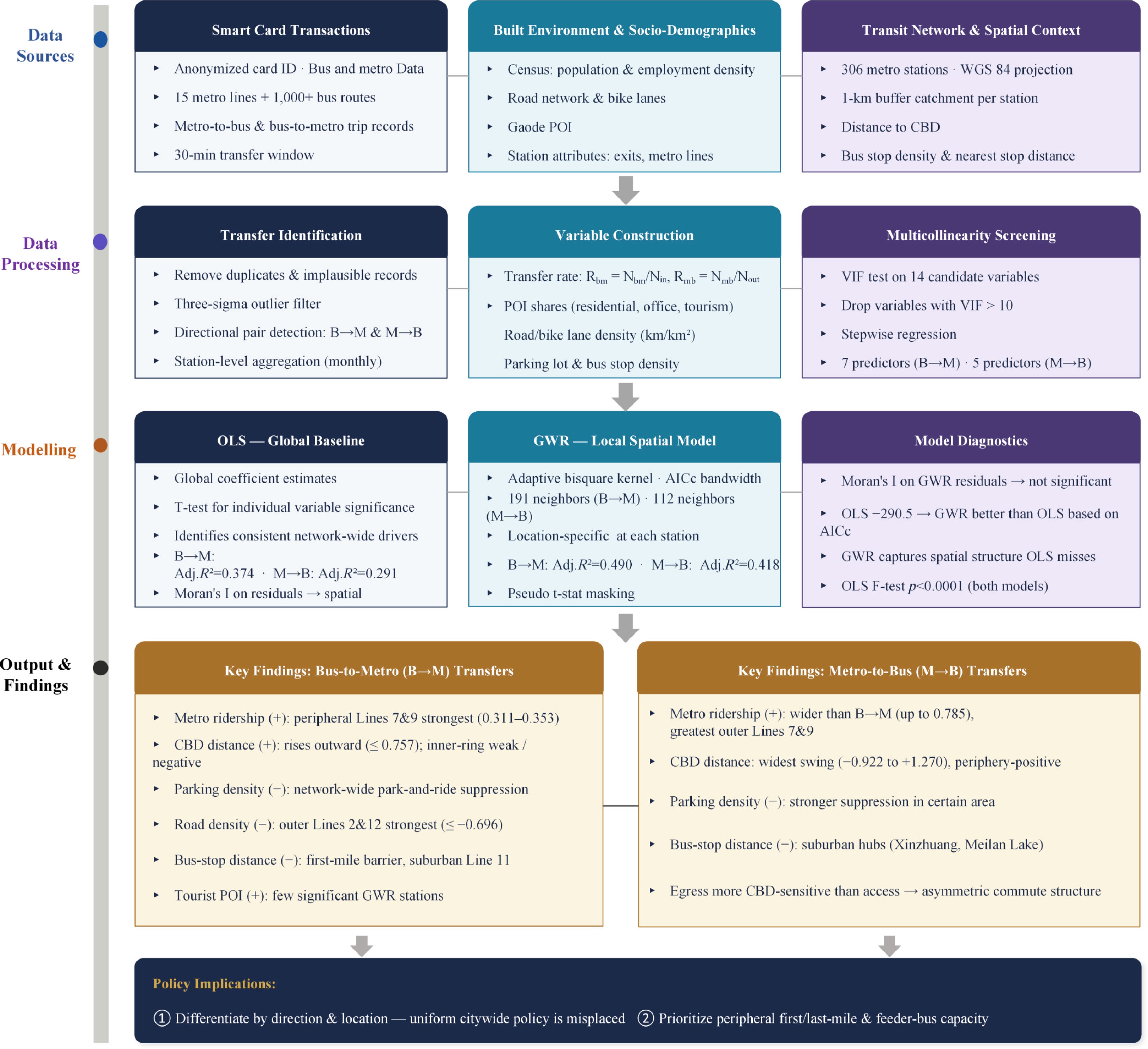
Figure 1.
General research framework for analyzing spatial heterogeneity in metro–bus transfer behavior.
-
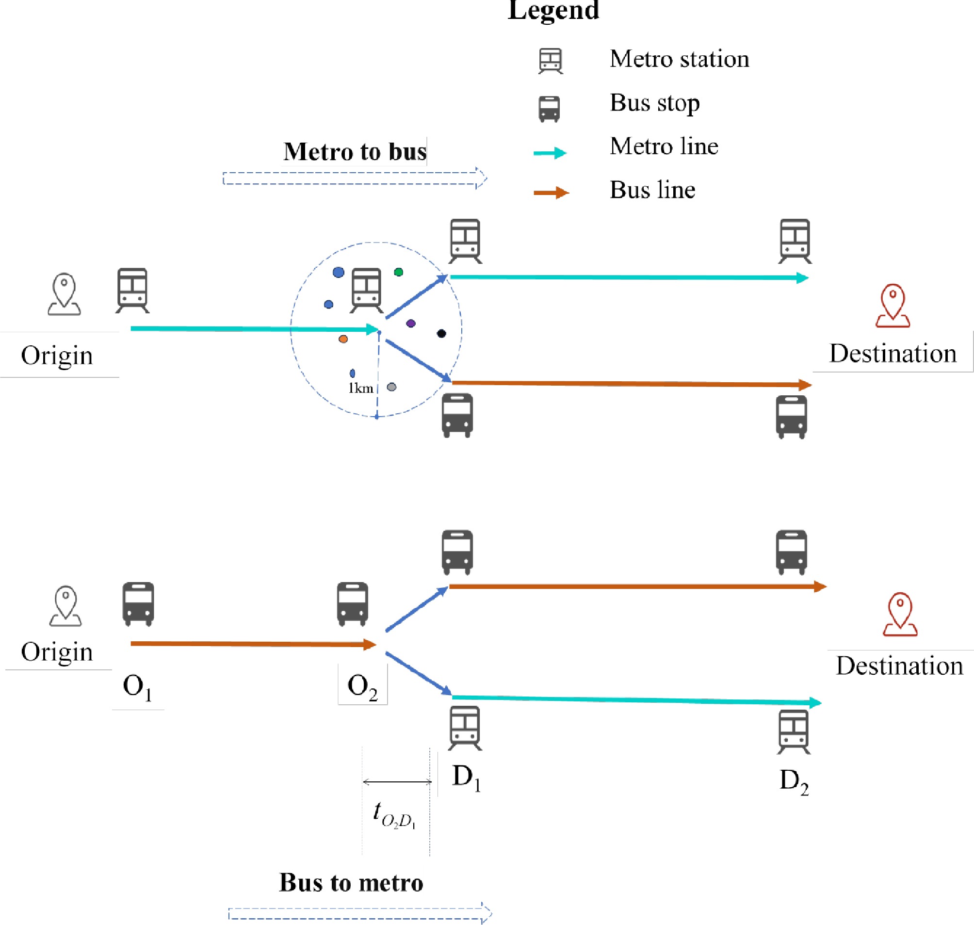
Figure 2.
Defining a metro–bus transfer: a 30-min window linking trip legs across modes.
-
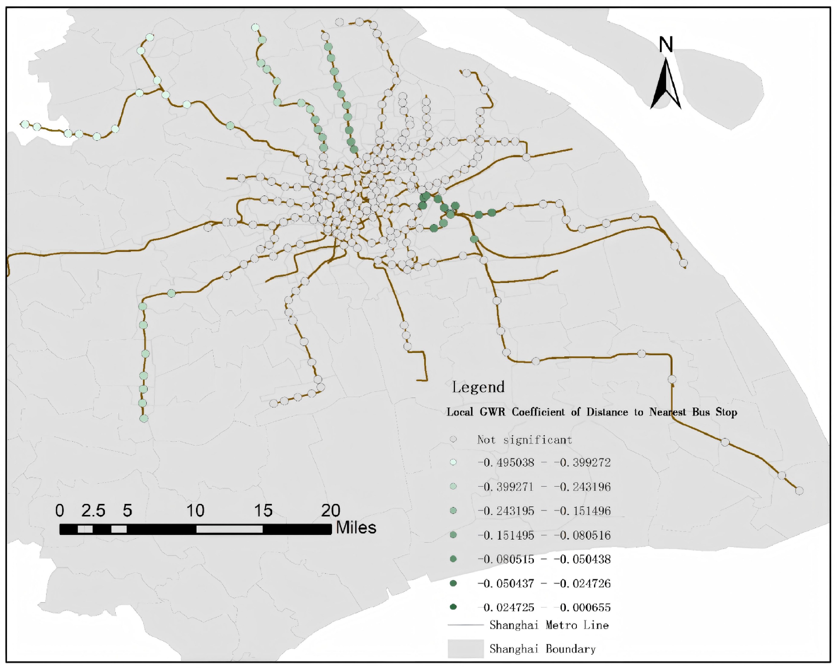
Figure 3.
Local GWR coefficient of nearest bus stop distance on bus-to-metro transfer rates.
-
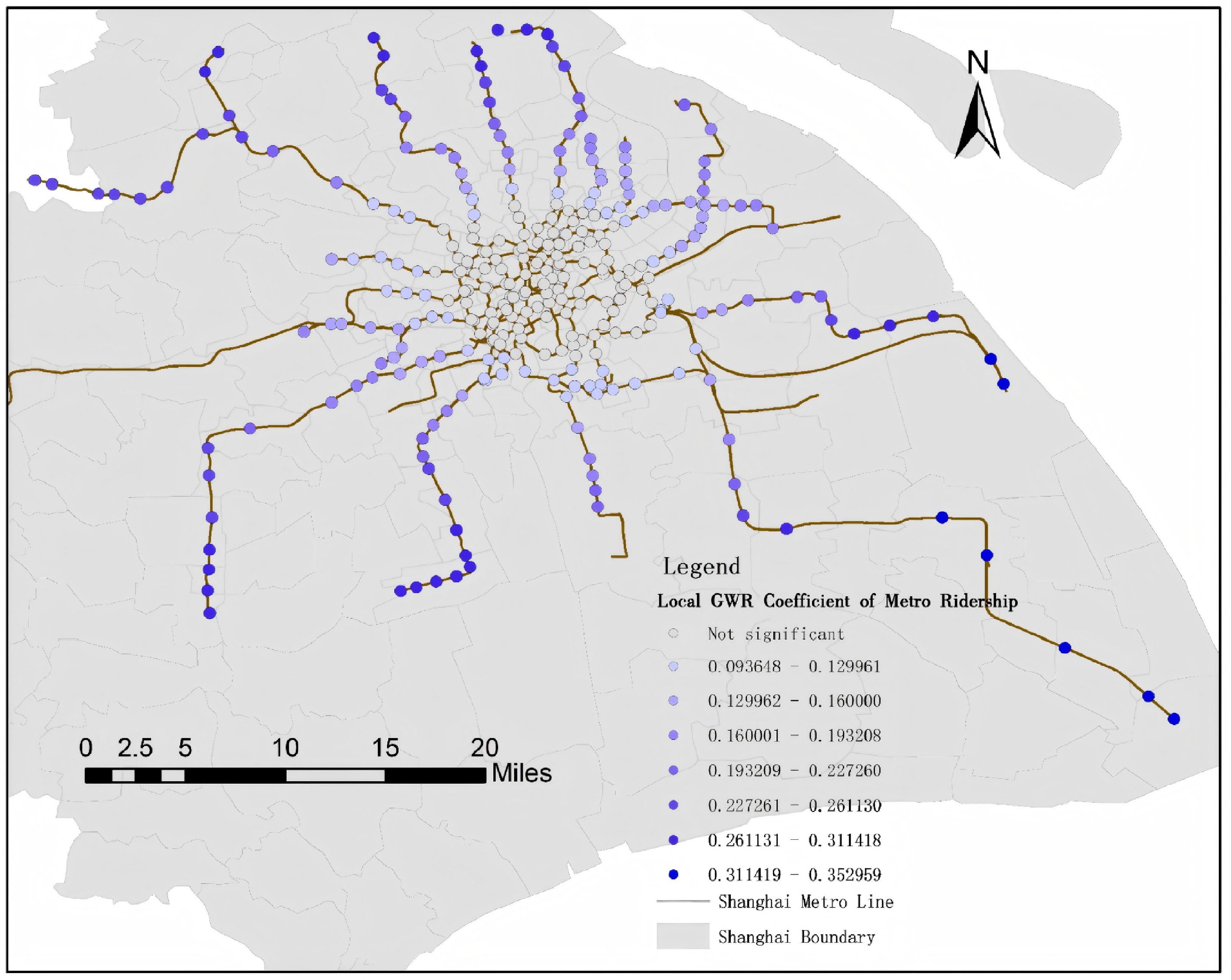
Figure 4.
Local GWR coefficient of metro ridership on bus-to-metro transfer rates.
-
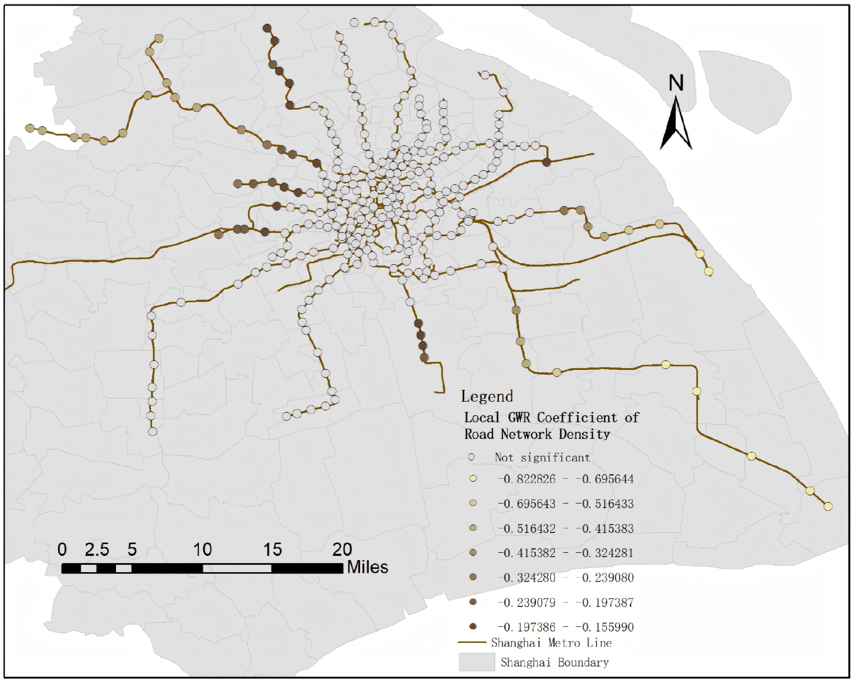
Figure 5.
Local GWR coefficient of road network density on bus-to-metro transfer rates.
-
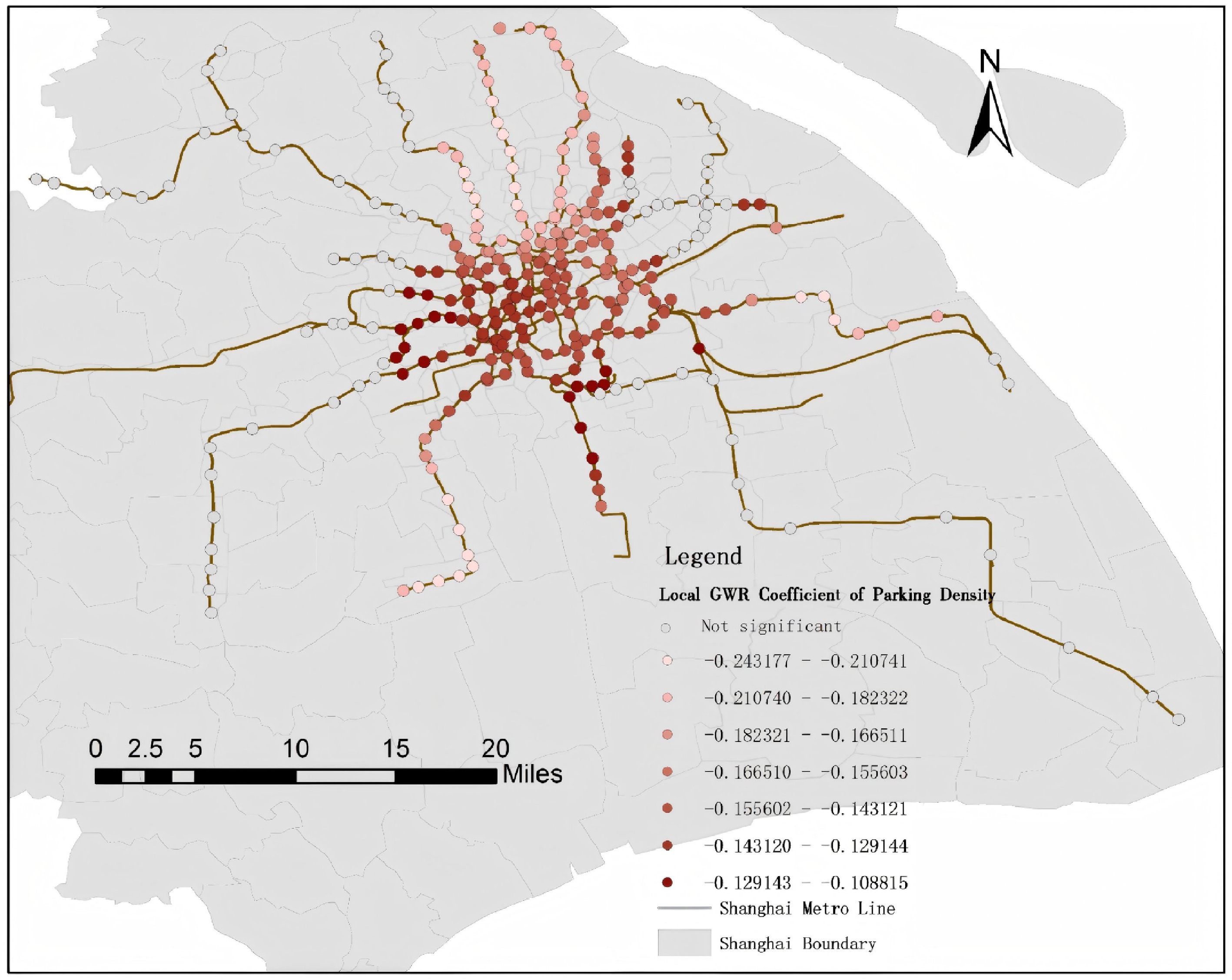
Figure 6.
Local GWR coefficient of parking density on bus-to-metro transfer rates.
-
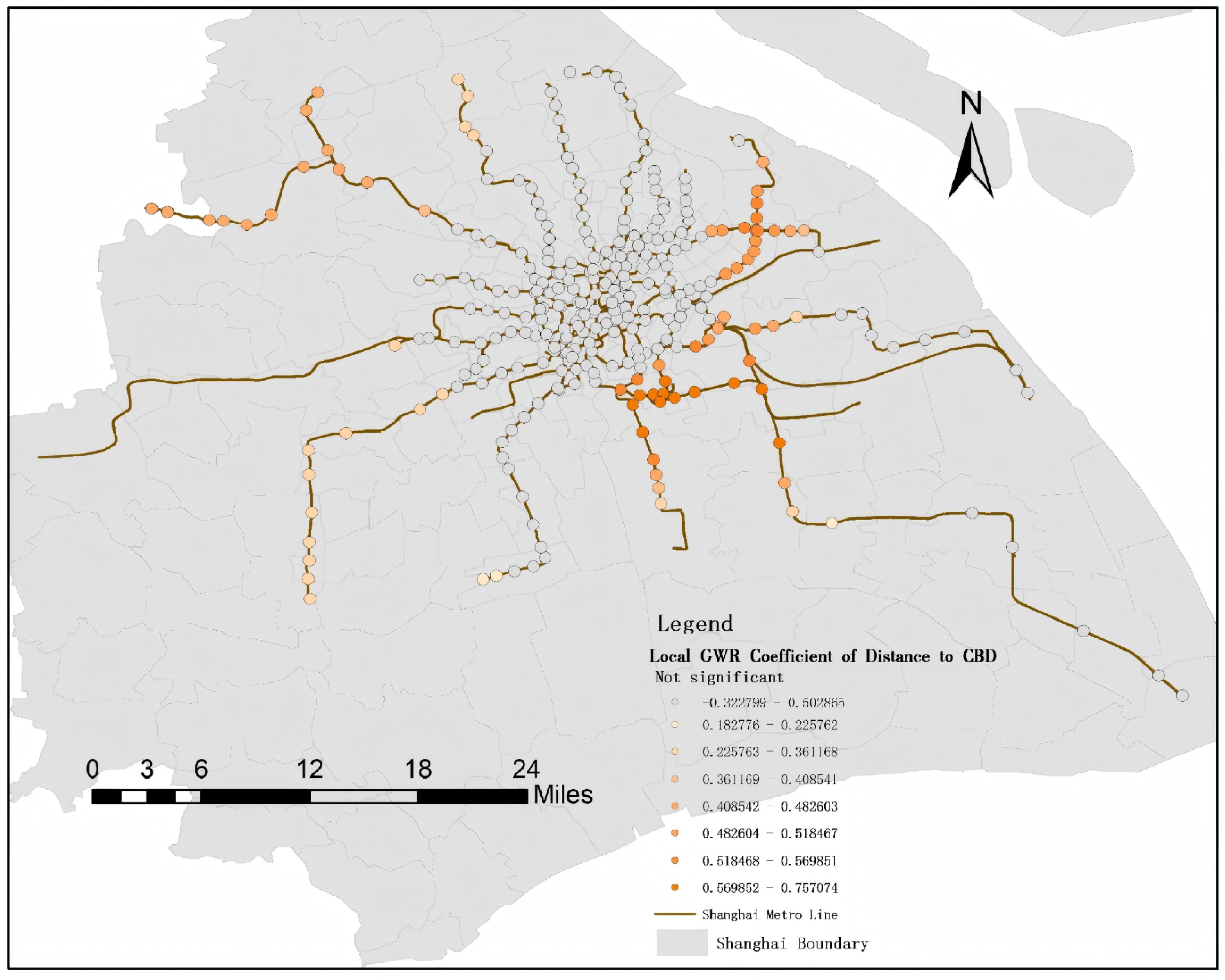
Figure 7.
Local GWR coefficient of distance to CBD on bus-to-metro transfer rates.
-
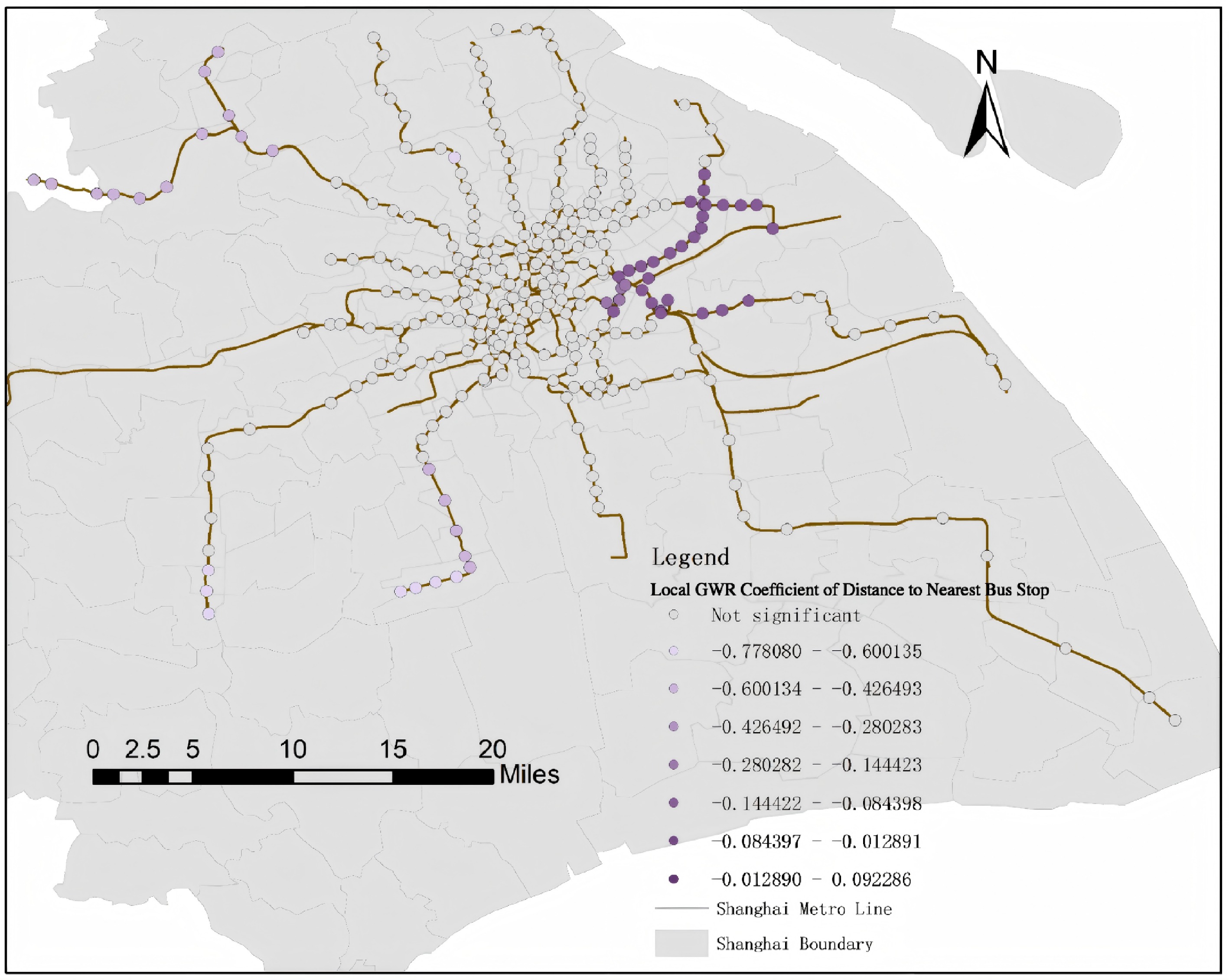
Figure 8.
Local GWR coefficient of distance to nearest bus stop on metro-to-bus transfer rates.
-
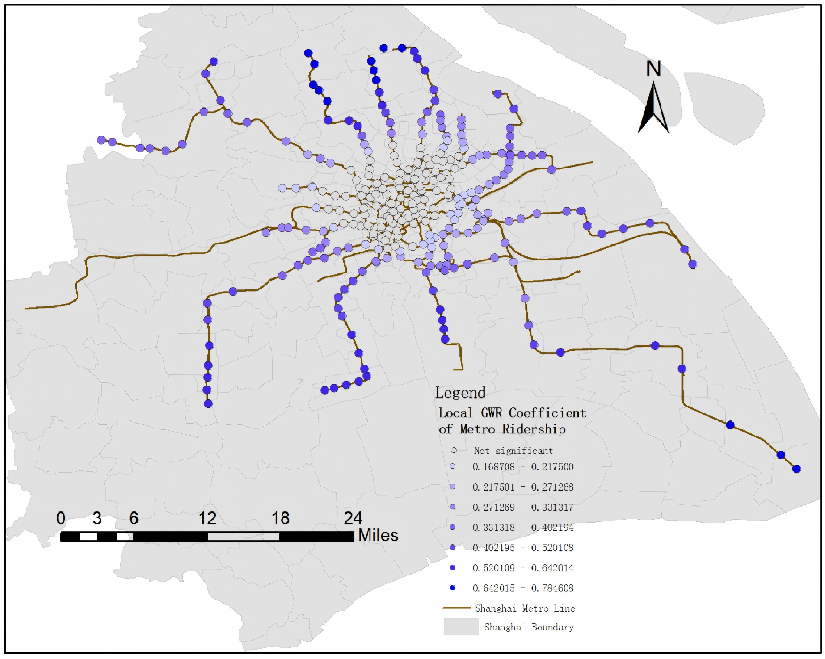
Figure 9.
Local GWR coefficient of metro ridership on metro-to-bus transfer rates.
-
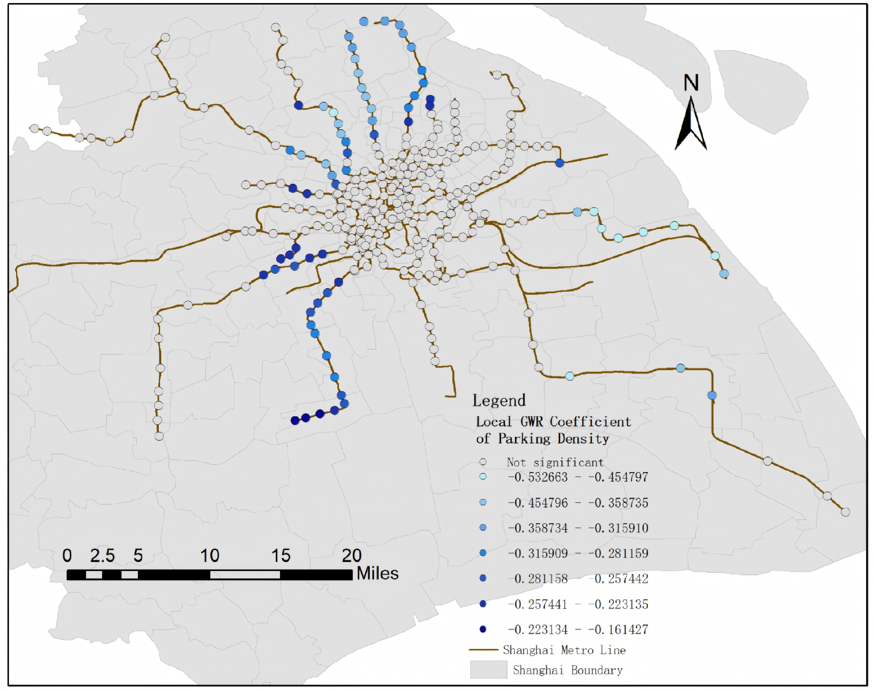
Figure 10.
Local GWR coefficient of parking density on metro-to-bus transfer rates.
-
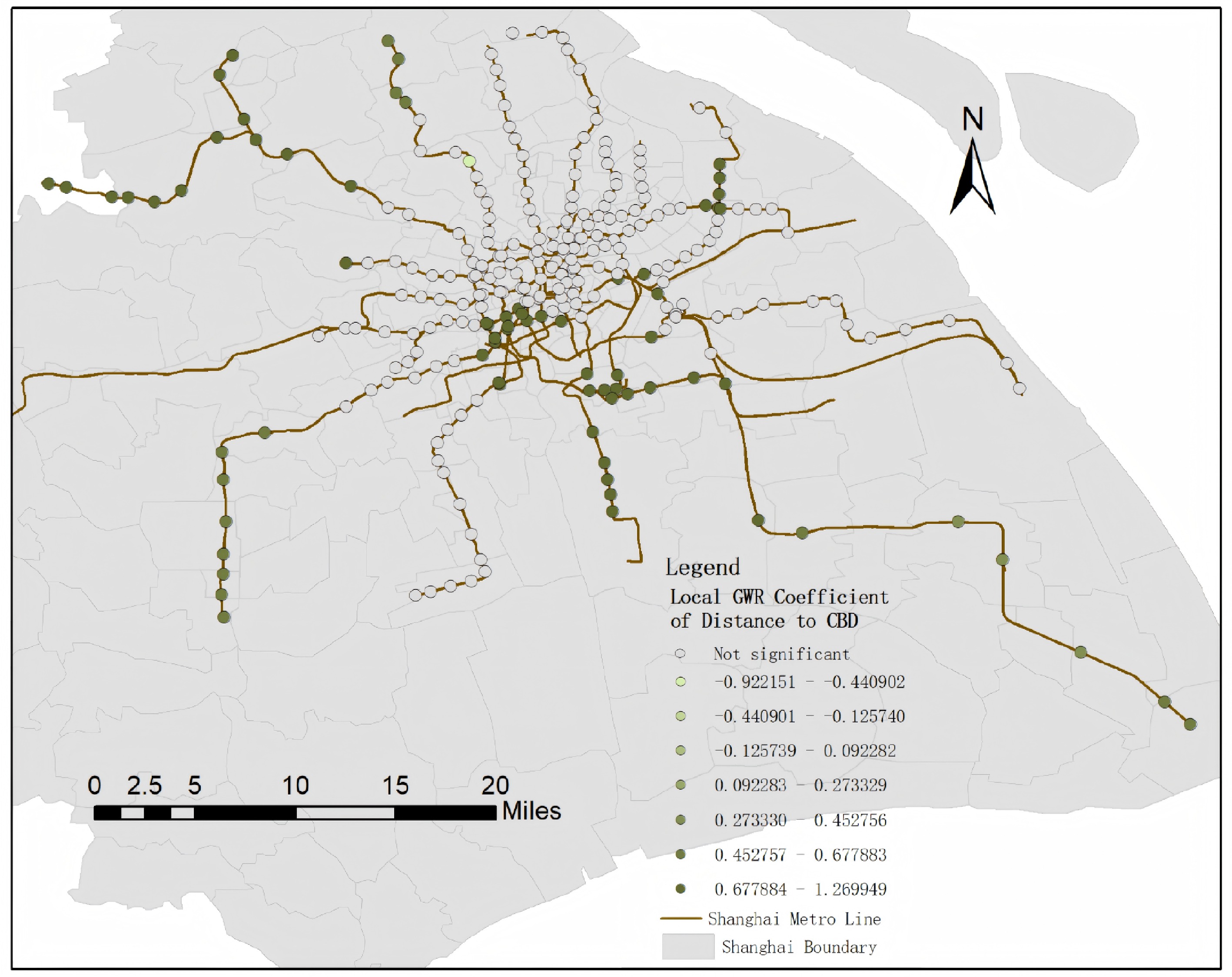
Figure 11.
Local GWR coefficient of distance to CBD on metro-to-bus transfer rates.
-
Category Variable Symbol Min Mean Max SD Dependent variables Bus $ \rightarrow $ $ R_{{{\mathrm{B}}\to {\mathrm{M}}}} $ 0.000296 0.122 0.696 0.123 Metro $ \rightarrow $ $ R_{{{\mathrm{M}}\to {\mathrm{B}}}} $ 0.000132 0.113 0.803 0.118 Transit service and station network Metro ridership (monthly) $ MR $ 1,171 436,923 2,567,207 387,063 Number of metro lines $ N_{\text{line}} $ 1 1.310 4 0.621 Number of station exits $ N_{\text{exit}} $ 1 5.143 20 2.826 Distance to nearest bus stop $ D_{\text{bus\_nn}} $ 0.003 0.256 1.872 0.326 Bus stop density $ D_{\text{bus}} $ 0 7.065 15.924 3.153 Built environment Parking density $ D_{\text{par}} $ 0 5.118 13.113 3.771 Bicycle lane density $ D_{\text{bld}} $ 0 0.452 4.023 0.863 Road network density $ D_{\text{road}} $ 0.036 12.791 32.331 5.540 Distance to CBD $ D_{\text{CBD}} $ 0.552 13.735 65.984 10.324 Residential POI share $ P_{\text{res}} $ 0.215 0.472 0.798 0.096 Office POI share $ P_{\text{off}} $ 0 0.101 0.288 0.029 Tourism POI share $ P_{\text{tour}} $ 0 0.328 0.667 0.060 Population density (buffer) $ P_{\text{pop}} $ 56 18,851.271 44,682 12,126.491 Employment density (buffer) $ P_{\text{job}} $ 0.080 285.476 905.573 246.295 SD, standard deviation; POI, point of interest; CBD, central business district. #, number (count). Transfer rates and POI shares are expressed as ratios (0–1), not percentages. Metro ridership is the total number of entries recorded at the station over the 1-month study period (April 2015). All built-environment and socio-demographic indicators are measured within a 1 km buffer around each metro station. Table 1.
Definitions and descriptive statistics of the variables.
-
Variable Coefficient t-statistic p-value Significance Road network density −0.139395 −2.187172 0.029495 ** Distance to nearest bus stop −0.074204 −1.864957 0.063174 * Distance to CBD 0.230025 3.210951 0.001468 *** Population densitya −0.029297 −0.622181 0.534300 ns Proportion of tourist POIs 0.318515 2.044617 0.041763 ** Parking density −0.136822 −3.438710 0.000681 *** Metro ridership 0.154115 3.837729 0.000161 *** ***, **, and * indicate that the coefficient is statistically significant at the 1%, 5%, and 10% levels, respectively (i.e., p < 0.01, p < 0.05, and p < 0.10); ns indicates not significant (p ≥ 0.10). a Population density was retained in the OLS results for transparency, but excluded from the GWR estimation due to its insignificant OLS t-statistic. Table 2.
OLS coefficient estimates and t-tests (
$ R_{{\mathrm{B}} \rightarrow {\mathrm{M}}} $ -
Variable Coefficient t-statistic p-value Significance Distance to CBD 0.336207 2.407780 0.016641 ** Population density −0.047775 −0.761604 0.446886 ns Distance to nearest bus stop −0.122878 −2.490553 0.013285 ** Parking density −0.160087 −3.049310 0.002507 *** Metro ridership 0.266319 4.689708 0.000006 *** ***, **, and * indicate that the coefficient is statistically significant at the 1%, 5%, and 10% levels, respectively (i.e., p < 0.01, p < 0.05, and p < 0.10); ns indicates not significant (p ≥ 0.10). Table 3.
OLS coefficient estimates and t-tests (
$ R_{{\mathrm{M}} \rightarrow {\mathrm{B}}} $ -
Model Moran's $ I $ $ Z $ p-value Significance OLS (B $ \rightarrow $ 0.113058 4.451014 < 0.00001 *** OLS (M $ \rightarrow $ 0.123467 4.858613 < 0.00001 *** ***, **, and * indicate statistical significance at the 1%, 5%, and 10% levels, respectively; ns indicates not significant (p ≥ 0.10). Table 4.
Global Moran's
$ I $ -
Model Moran's $ I $ $ Z $ p-value Significance GWR (B $ \rightarrow $ −0.003062 0.016194 0.987079 ns GWR (M $ \rightarrow $ −0.012077 −0.632434 0.527103 ns ***, **, and * indicate statistical significance at the 1%, 5%, and 10% levels, respectively; ns indicates not significant (p ≥ 0.10). Table 5.
Global Moran's
$ I $ -
Variable Moran's $ I $ Expected index $ Z $ p-value Significance Metro ridership 0.258069 −0.003279 10.05420 < 0.000001 *** Distance to nearest bus stop 0.452975 −0.003279 17.57602 < 0.000001 *** Distance to CBD 0.957835 −0.003279 36.96441 < 0.000001 *** Population density 0.786053 −0.003279 30.08828 < 0.000001 *** Tourist POI proportion 0.383708 −0.003279 15.59166 < 0.000001 *** Road network density 0.646344 −0.003279 24.85657 < 0.000001 *** Parking lot density 0.693274 −0.003279 24.90747 < 0.000001 *** ***, **, and * indicate statistical significance at the 1%, 5%, and 10% levels, respectively; ns indicates not significant (p ≥ 0.10). Table 6.
Moran's
$ I $ $ R_{{\mathrm{B}} \rightarrow {\mathrm{M}}} $ -
Variable Moran's $ I $ Expected index $ Z $ p-value Significance Metro ridership 0.258069 −0.003279 10.05420 < 0.000001 *** Distance to CBD 0.957835 −0.003279 36.96441 < 0.000001 *** Parking lot density 0.693274 −0.003279 24.90747 < 0.000001 *** Distance to nearest bus stop 0.452975 −0.003279 17.57602 < 0.000001 *** Population density 0.786053 −0.003279 30.08828 < 0.000001 *** ***, **, and * indicate statistical significance at the 1%, 5%, and 10% levels, respectively; ns indicates not significant (p ≥ 0.10). Table 7.
Moran's
$ I $ $ R_{{\mathrm{M}} \rightarrow {\mathrm{B}}} $ -
Model $ R^{2} $ Adj. $ R^{2} $ AICc $ F $ p-value Significance OLS 0.388 0.374 −438.513 26.992 < 0.000001 *** GWRa 0.548 0.490 −486.286 – – – ***, **, and * indicate statistical significance at the 1%, 5%, and 10% levels, respectively; ns indicates not significant (p ≥ 0.10); '–' indicates not applicable, as the GWR model does not report a global $ F $ Table 8.
GWR outperforms OLS in explaining bus-to-metro transfer rates (
$ R_{{\mathrm{B}} \rightarrow {\mathrm{M}}} $ -
Model $ R^{2} $ Adj. $ R^{2} $ AICc $ F $ p-value Significance OLS 0.303 0.291 −290.548 26.064 < 0.000001 *** GWRa 0.497 0.418 −329.746 – – – ***, **, and * indicate statistical significance at the 1%, 5%, and 10% levels, respectively; ns indicates not significant (p ≥ 0.10); '–' indicates not applicable, as the GWR model does not report a global $ F $ Table 9.
GWR outperforms OLS in explaining metro-to-bus transfer rates (
$ R_{{\mathrm{M}} \rightarrow {\mathrm{B}}} $
Figures
(11)
Tables
(9)