-
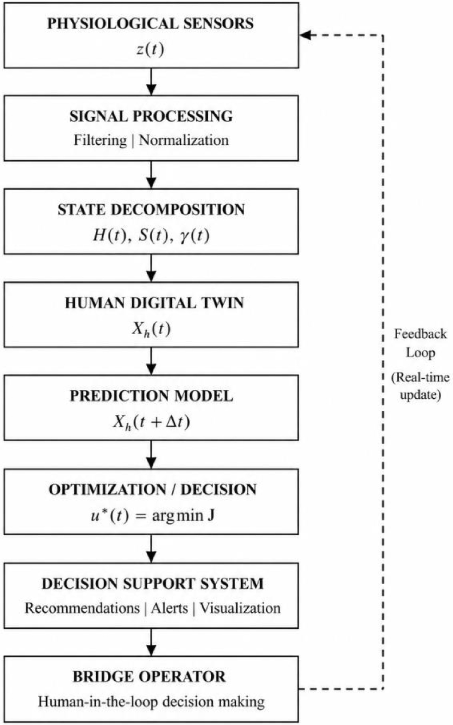
Figure 1.
Digital framework.
-
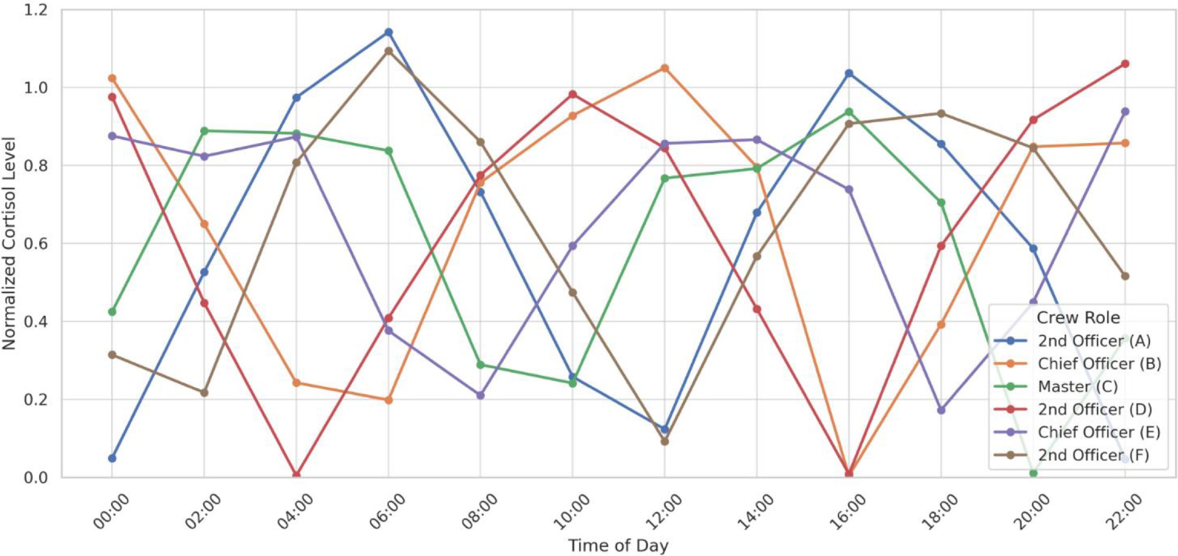
Figure 2.
Distribution of circadian rhythms in crew members based on t-test cortisol concentration results.
-
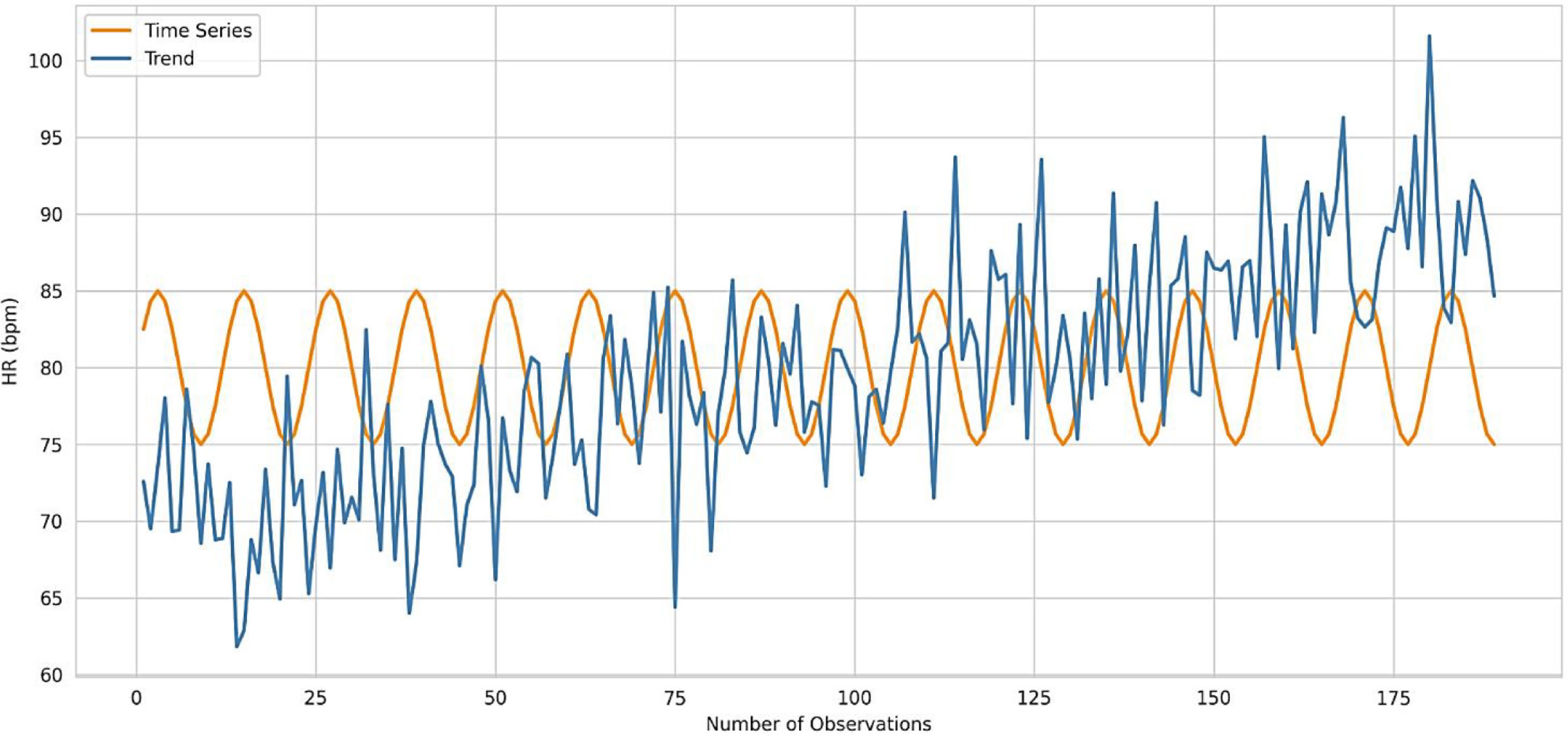
Figure 3.
Trend of the navigator's states.
-
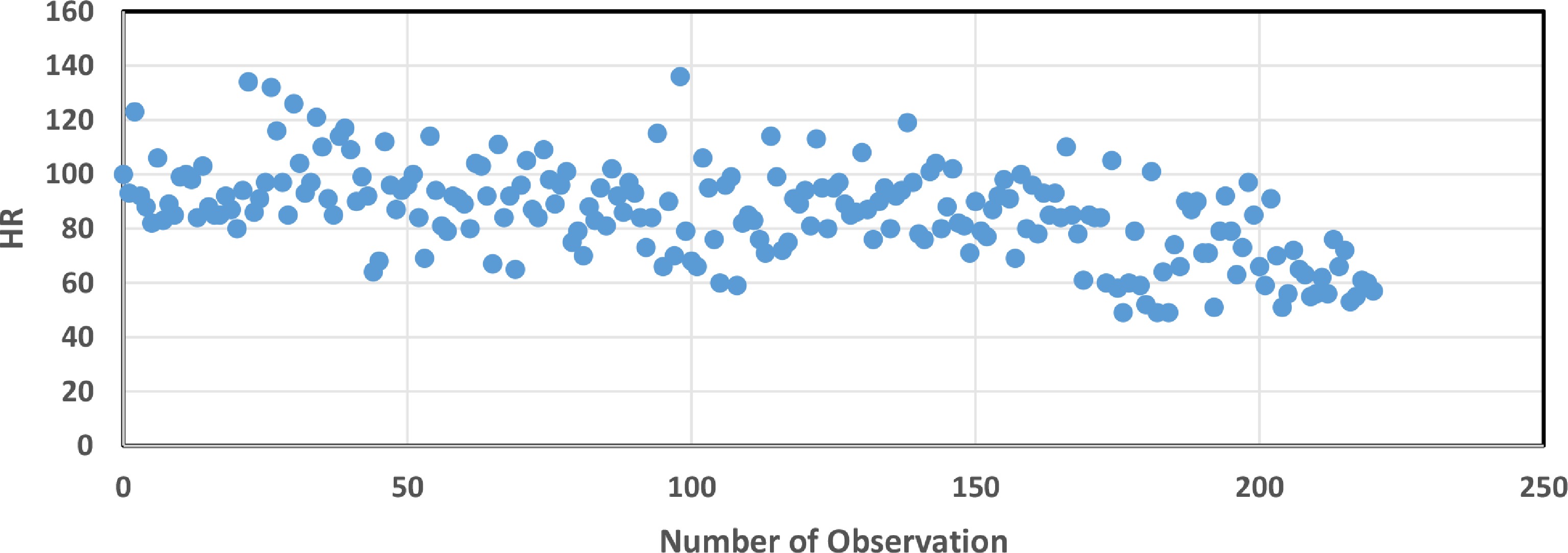
Figure 4.
Correlation field for yt.
-
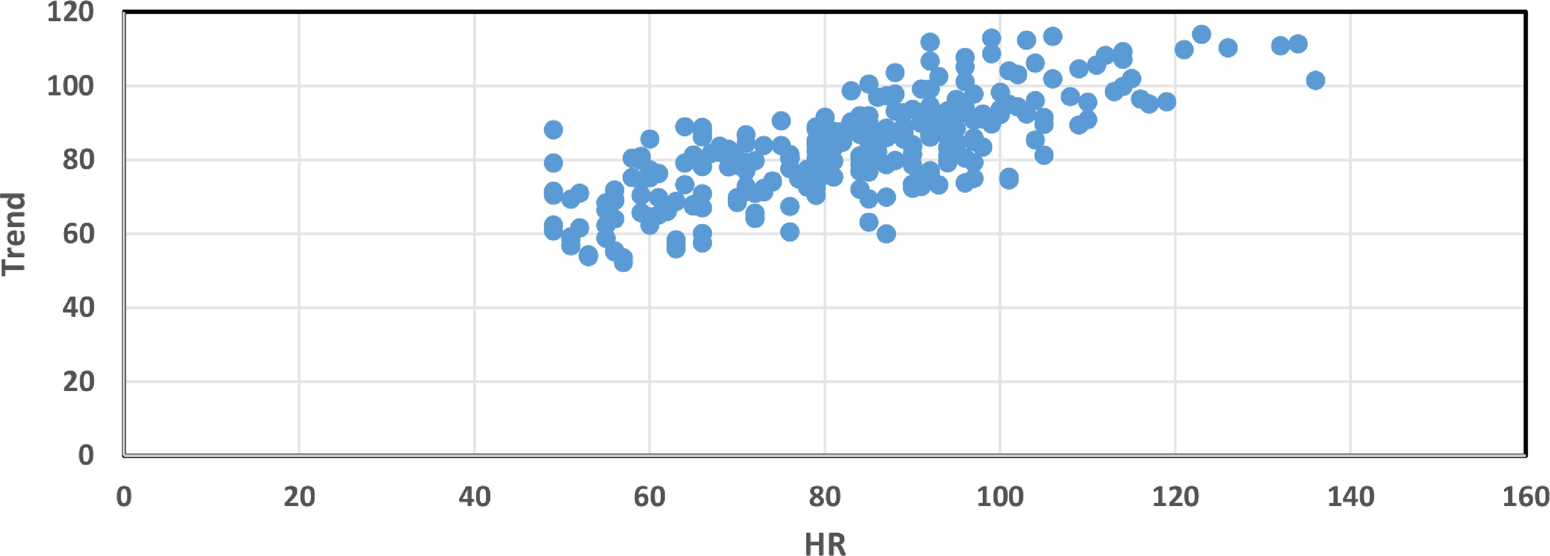
Figure 5.
Correlation field for
$ {y}_{T{{S}_{i}}} $ -
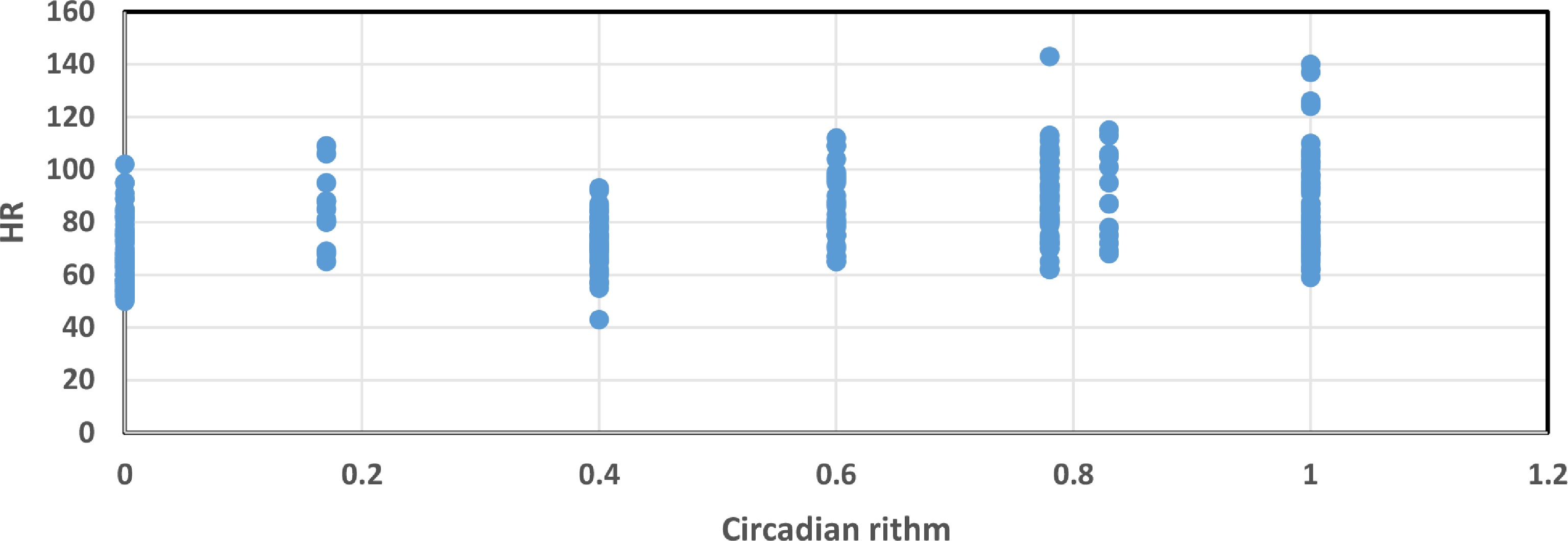
Figure 6.
Relationship between heart rate and circadian rhythm weighting.
-
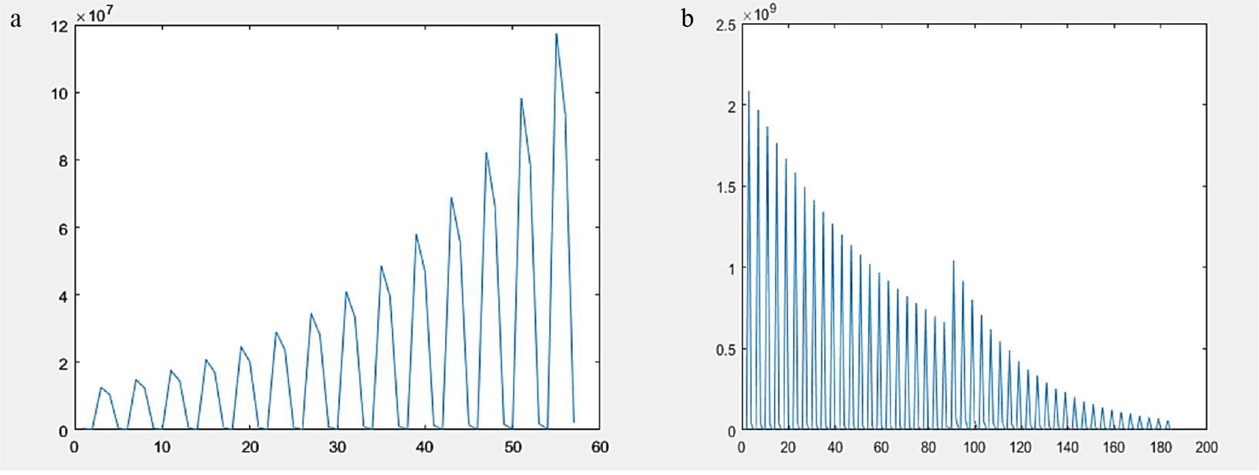
Figure 7.
Adaptation coefficient graph: (a) increasing trend; (b) decreasing trend.
-
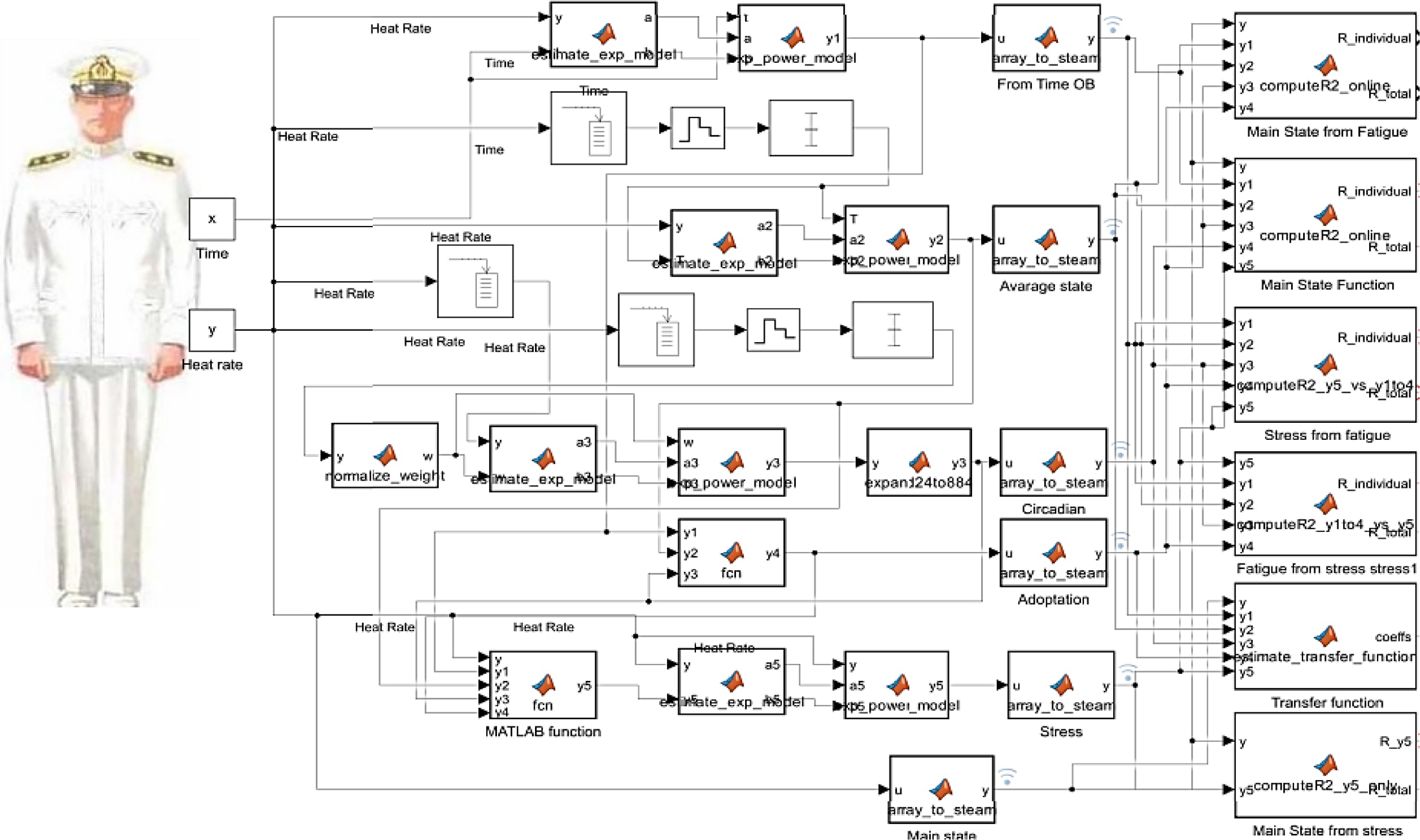
Figure 8.
Model of the monitoring and forecasting system for the psychophysiological states of the ship navigator.
-
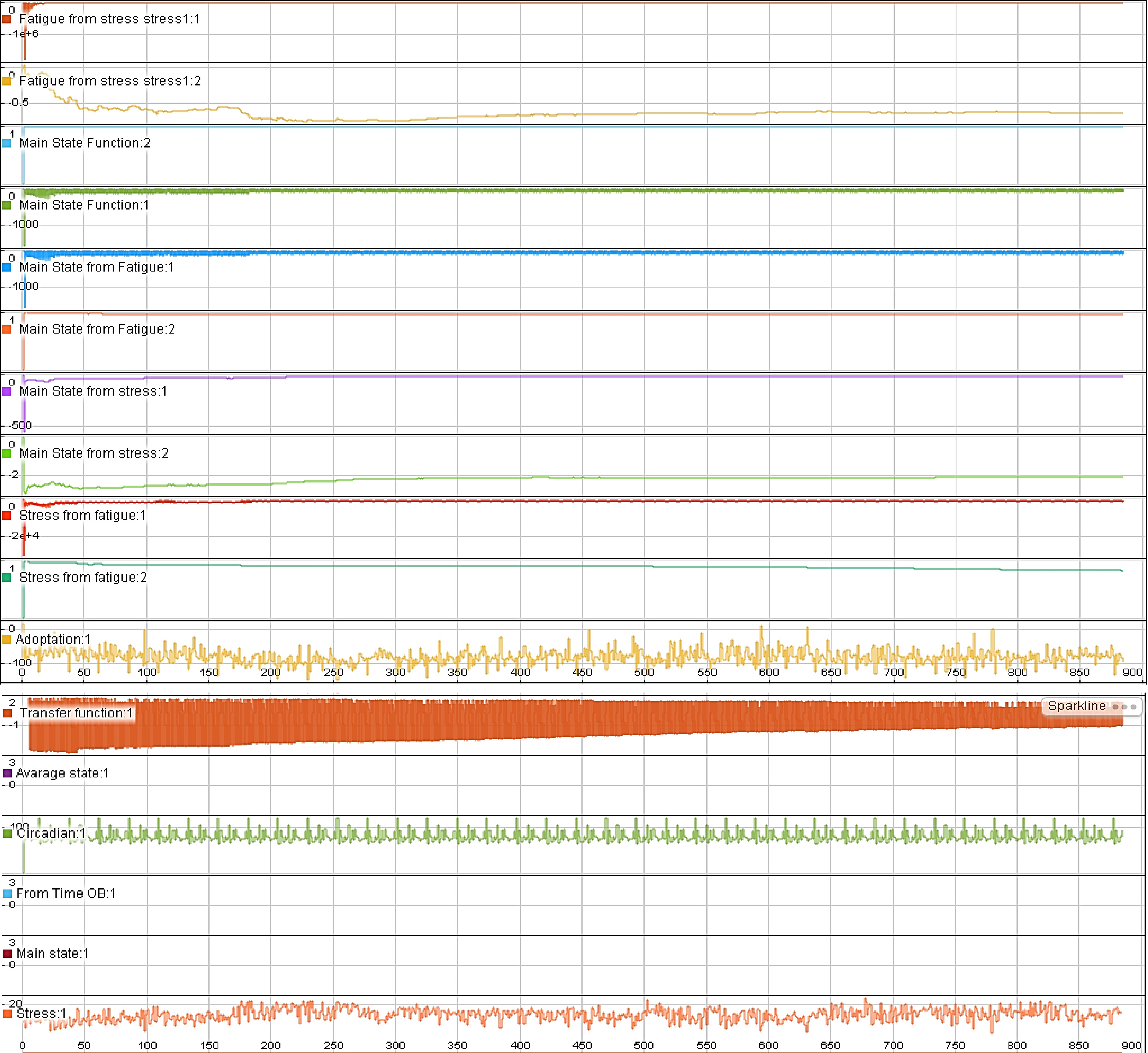
Figure 9.
Simulation of the state with predominance of fatigue.
-
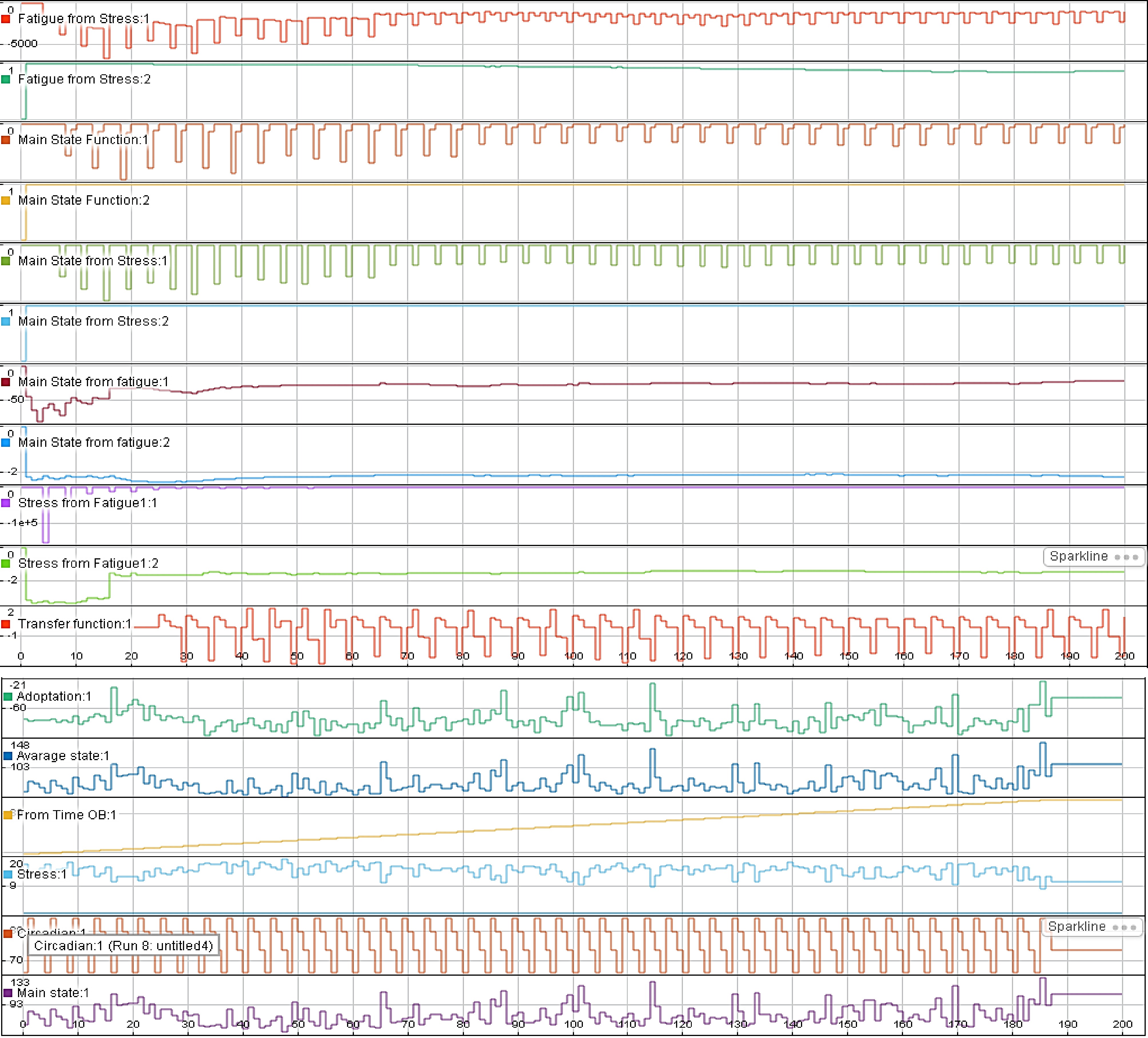
Figure 10.
Simulation of the state with predominance of stress.
-
Rank 2nd Officer (a) Ch. Officer (b) Master (c) 2nd Officer (d) Ch. Officer (e) Ch. Officer (f) 2nd Officer (g) 2nd Officer (a) − SZ NSZ NSZ NSZ NSZ NSZ Ch. Officer (b) SZ − NSZ UZ NSZ UZ SZ Master (c) NSZ NSZ − NSZ NSZ NSZ NSZ 2nd Officer (d) NSZ UZ NSZ − NSZ NSZ NSZ Ch. Officer (e) NSZ NSZ NSZ NSZ − NSZ NSZ Ch. Officer (f) NSZ ЗНВ NSZ NSZ NSZ − NSZ 2nd Officer (g) NSZ SZ NSZ NSZ NSZ NSZ − SZ - Significance Zone, NSZ - Non-significance Zone, UZ - Uncertainty Zone. Table 1.
Similarity of circadian rhythms according to the t-test.
-
Rank 2nd Officer (a) Ch. Officer (b) Master (c) 2nd Officer (d) Ch. Officer (e) Ch. Officer (f) 2nd Officer (g) R2 0.46 0.19 0.18 0.17 0.27 0.14 0.47 F 83.9 11.3 22.14 17.05 20.53 7.9 86.25 Table 2.
Coefficients of determination and F-test values for the experiment participants.
-
y t a b x y xy S ( x )2 S ( y )2 S ( x ) S ( y ) β A R R2 F 2nd Officer (a) 2.0082 −0.00076 110 1.925 208.612 4070 0.00807 63.797 0.0898 −0.54 3.18% 0.54 0.291 90.009 Ch. Officer (b) 1.8574 −0.00128 24 1.827 43.583 200 0.00796 14.142 0.0892 −0.203 3.96% 0.203 0.04131 2.025 Master (c) 1.8737 0.00021 93.5 1.893 177.64 2,945.22 0.00487 54.27 0.0698 0.163 2.97% 0.163 0.026 5.082 2nd Officer (d) 1.9049 0.0001 42 1.909 80.244 602 0.0682 24.536 0.0826 0.0299 3.45% 0.0299 0.000891 0.074 Ch. Officer (e) 1.8935 0.000839 29 1.918 55.844 270.67 0.00839 16.452 0.0916 0.151 3.99% 0.151 0.0227 1.277 Ch. Officer (f) 1.9618 −0.00117 24 1.934 46.176 200 0.00462 14.142 0.068 −0.243 2.57% 0.243 0.0592 2.957 2nd Officer (g) 1.876 −5.603 92 1.871 171.989 28.52 0.00757 53.404 0.087 −0.0344 3.77% 0.0344 0.0012 0.217 Table 3.
Estimated coefficients of the regression equation.
-
$ {{y}}_{{T}\cdot {{{S}}_{{i}}}} $ a b x y xy S(x)2 S(y)2 S(x) S(y) β A R R2 F 2nd Officer (a) 1.688 0.00281 85.814 1.929 166.325 289.64 0.00419 17.019 0.0648 0.737 1.80% 0.737 0.544 260.765 Ch. Officer (b) 1.7355 0.00144 68.551 1.834 126.039 214.08 0.0023 14.632 0.048 0.438 1.84% 0.438 0.192 11.176 Master (c) 1.7504 0.00176 79.266 1.89 150.144 181.04 0.00202 13.455 0.0449 0.528 1.60% 0.528 0.279 71.941 2nd Officer (d) 1.8459 0.000844 82.588 1.916 158.411 243.96 0.00101 15.619 0.0319 0.414 1.22% 0.414 0.171 17.153 Ch. Officer (e) 1.7984 0.00149 84.596 1.925 163.337 341.19 0.00278 18.471 0.0527 0.523 2.03% 0.523 0.274 20.714 Ch. Officer (f) 1.8777 0.000698 86.939 1.938 168.661 202.34 0.000672 14.225 0.0259 0.383 1.02% 0.383 0.147 8.072 2nd Officer (g) 1.7222 0.00205 75.859 1.878 142.973 245.31 0.00286 15.662 0.0535 0.602 1.93% 0.602 0.363 104.097 Table 4.
Estimated coefficients of the regression equation.
-
уc a b x y xy S(x)2 S(y)2 S(x) S(y) β A R R2 F 2nd Officer (a) 1.882 0.1009 0.422 1.925 0.825 0.13 0.00807 0.363 0.0898 0.408 3.34% 0.408 0.167 43.811 Ch. Officer (b) 1.7723 0.09586 0.556 1.827 1.048 0.14 0.00796 0.368 0.0892 0.395 3.76% 0.395 0.156 8.694 Master (c) 1.8406 0.08972 0.588 1.893 1.125 0.14 0.00487 0.372 0.0698 0.478 2.42% 0.478 0.228 55.028 2nd Officer (d) 1.8621 0.09085 0.518 1.909 1.001 0.12 0.00682 0.353 0.0826 0.389 3.13% 0.389 0.151 14.772 Ch. Officer (e) 1.8419 0.125 0.607 1.918 1.182 0.14 0.00839 0.375 0.0916 0.512 3.44% 0.512 0.262 19.513 Ch. Officer (f) 1.9095 0.056 0.433 1.934 0.847 0.15 0.00462 0.39 0.068 0.321 2.65% 0.321 0.103 5.411 2nd Officer (g) 1.8072 0.1176 0.544 1.871 1.035 0.14 0.00757 0.38 0.087 0.514 3.23% 0.514 0.264 65.575 Table 5.
Estimated coefficients of the regression equation.
-
y b0 b1 b2 b3 ԑ/Y A Se2 R2 F 2nd Officer (a) 0.4845 −0.00203 1.611 0.9893 24.62 11.09% 28,537.288 0.6 108.993 Ch. Officer (b) 0.4573 0.00149 −2.7542 1.0138 7.682 15.36% 8,453.35 0.44 12.048 Master (c) 3.9055 −0.0129 −0.7099 0.9859 20.067 10.62% 24,409.705 0.3941 40.105 2nd Officer (d) 1.3395 0.00619 1.4031 0.9713 20.796 14.34% 31,341.188 0.4841 44.108 Ch. Officer (e) 0.3255 −0.00137 1.1833 0.9908 5.547 11.09% 8,470.239 0.511 16.024 Ch. Officer (f) 33.9381 0.07623 12.8967 0.4795 8.787 15.42% 14,024.849 0.2788 6.831 2nd Officer (g) −1.1437 −0.00045 −0.2643 1.0145 23.554 12.66% 28,909.747 0.4343 46.579 Table 6.
Estimated coefficients of the multiple regression equation.
-
Rank A R2 2nd Officer (a) 2.89 0.54 Ch. Officer (b) 2.76 0.115 Master (c) 2.38 0.303 2nd Officer (d) 3.11 0.153 Ch. Officer (e) 3.43 0.277 Ch. Officer (f) 2.49 0.198 2nd Officer (g) 2.92 0.379 Table 7.
Assessment of the accuracy of fatigue-related factors' influence on the navigator's overall condition.
-
Rank ast bst A R2 2nd Officer (a) 1.5385 0.000585 0.68 0.027 Ch. Officer (b) 1.1455 0.00642 1.64 0.887 Master (c) 0.9162 0.0082 3.24 0.757 2nd Officer (d) 1.0212 0.00799 1.43 0.929 Ch. Officer (e) 0.9576 0.00789 2.95 0.857 Ch. Officer (f) 1.2038 0.00646 0.71 0.964 2nd Officer (g) 0.2027 0.000766 6.04 0.05 Table 8.
Estimated parameters of the relationship between overall condition and the stress component.
-
Rank R2 rX1 rX2 rX3 rX4 β1 β2 β3 β4 2nd Officer (a) 0.6 −0.78 −0.54 0.031 −0.54 −0.75 −0.032 0.0506 0 Ch. Officer (b) 0.33 0.073 0.073 0.39 −0.073 34.39 0 0.992 −35.13 Master (c) 0.06 −0.075 0.18 0.21 0.18 −0.219 11.259 0.0004 −10.984 2nd Officer (d) 0.12 0.0766 0.34 0.32 0.34 0.154 −40.99 0.506 40.83 Ch. Officer (s) 0.1146 0.0462 0.3 0.33 0.3 0.0838 −0.197 0.51 1.2Е-5 Ch. Officer (f) 0.08 0.11 0.241 0.240 0.242 0.385 −52.38 0.433 52.06 2nd Officer (g) 0.9968 0.988 0.0685 0.054 0.0685 0.998 0.0096 −0.00419 0 Table 9.
Indicators of the stress component's dependence on fatigue-associated factors.
-
Rank R2 rX1 rX2 rX3 rX4 rX5 β1 β2 β3 β4 β5 2nd Officer (a) 0.946 −0.019 0.55 0.74 0.45 0.742 0.999 0.843 0.687 0.0048 0 Ch. Officer (b) 0.985 0.96 0.34 0.34 0.57 0.42 0.94 −0.98 0 −0.02 1.263 Master (c) 0.977 0.91 0.2 0.53 0.45 0.53 0.857 0.125 1.773 0.0176 −1.459 2nd Officer (d) 0.968 0.98 0.083 0.41 0.39 0.41 0.95 −0.0247 6.333 −0.143 −6.102 Ch. Officer (e) 0.975 0.96 0.12 0.52 0.51 0.52 0.886 0.0227 0.37 −0.131 2E-6 Ch. Officer (f) 0.971 0.97 0.26 0.38 0.3 0.38 0.973 0.119 −3.05 0.0213 3.18 2nd Officer (g) 0.372 0.035 −0.0347 0.6 0.42 0.6 −1.177 −1.172 0.606 −0.00488 2Е-6 Table 10.
Indicators of the dependence of overall conditions on the stress component and fatigue-associated factors.
Figures
(10)
Tables
(10)