-
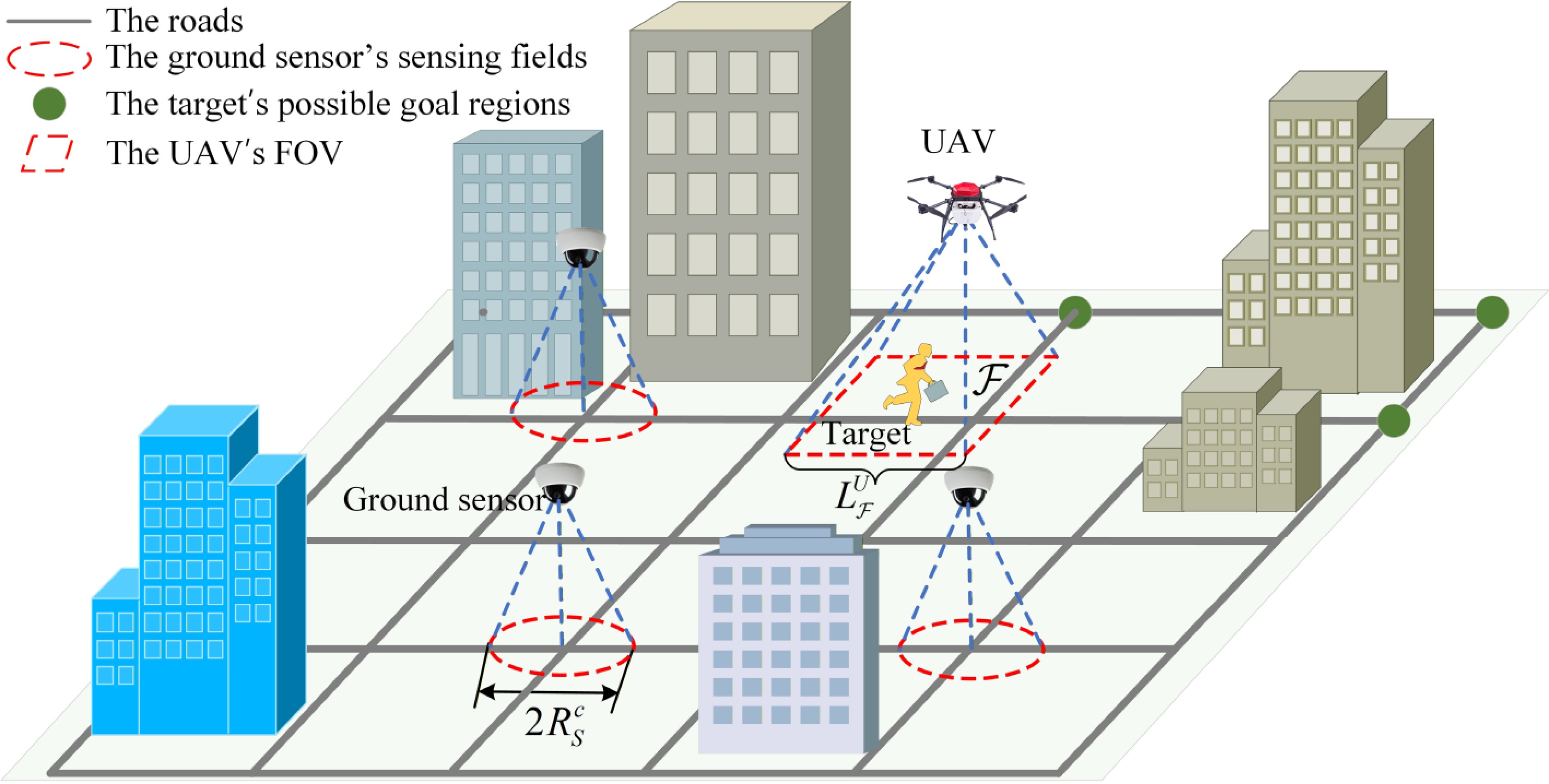
Figure 1.
Schematic diagram of the problem scenario.
-
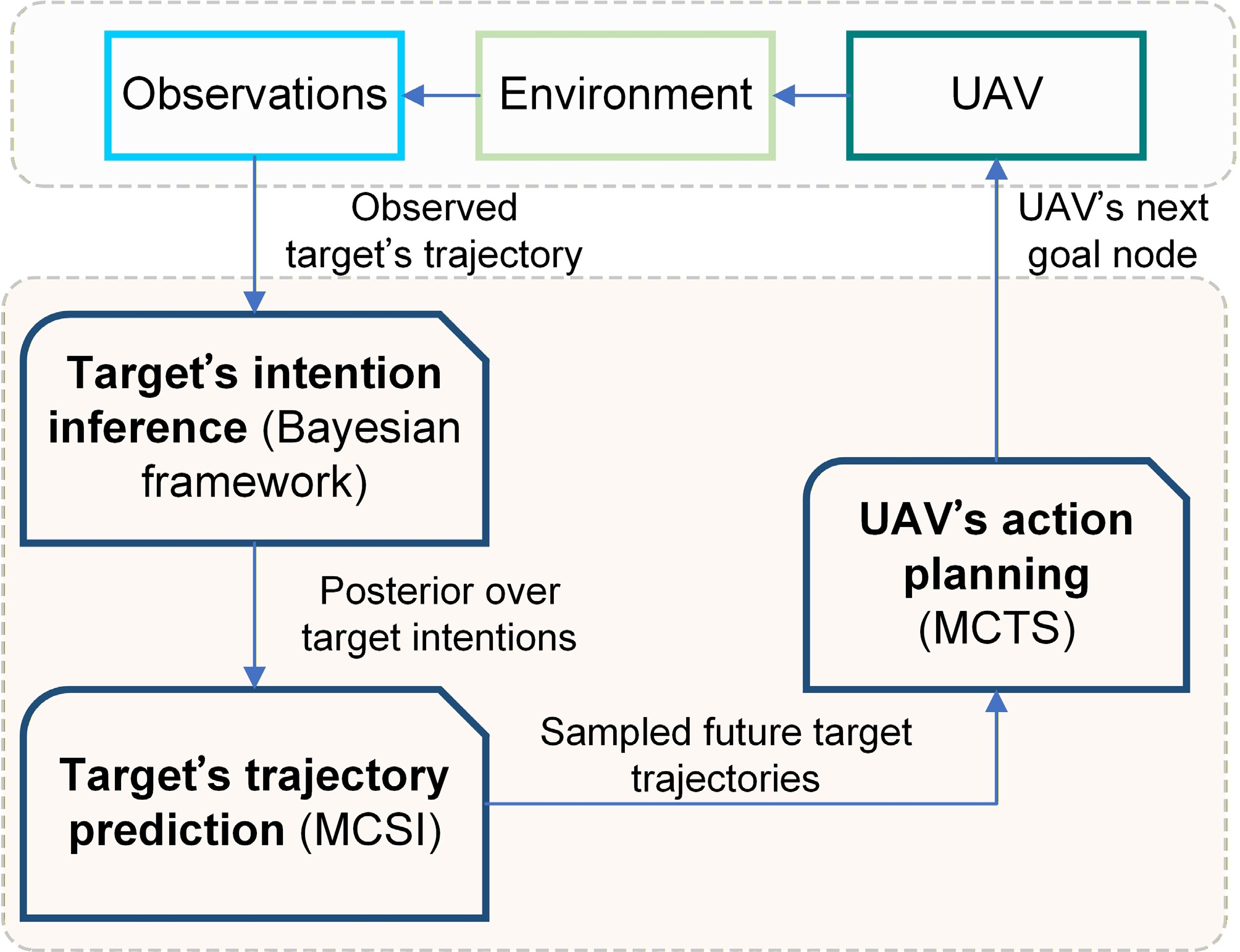
Figure 2.
System framework.
-
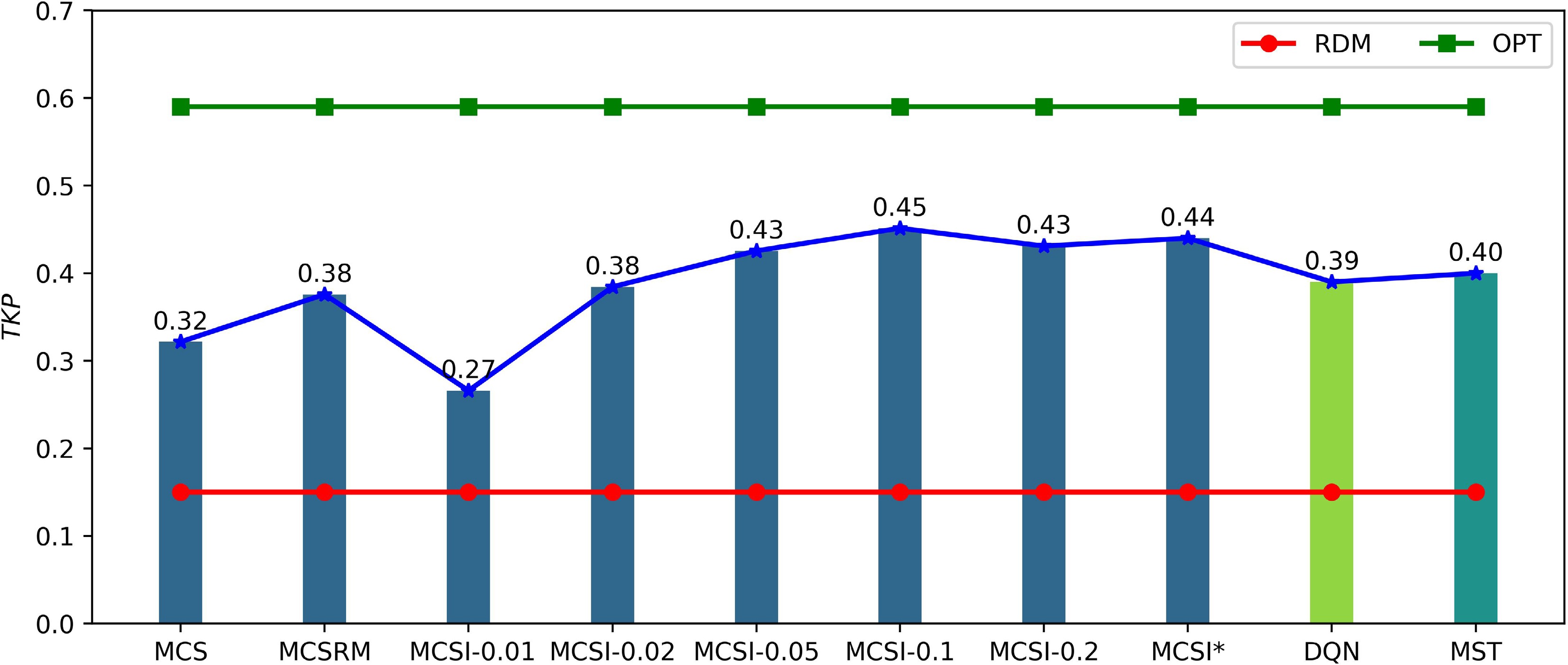
Figure 3.
The tracking performance of different methods.
-
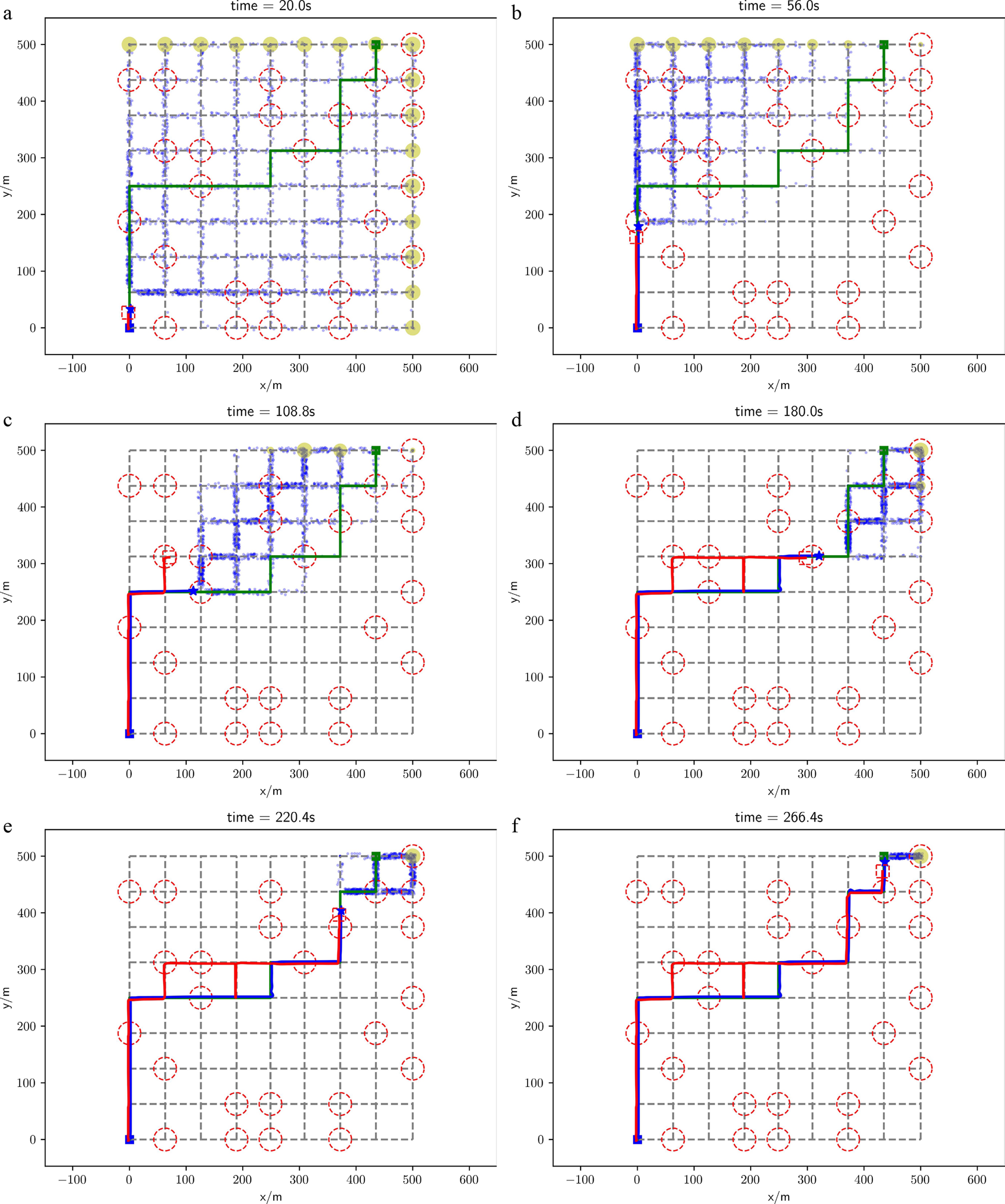
Figure 4.
Target tracking process in a test experiment. The target prediction method is MCSI*, and the UAV planning method is the MCTS-based planning method. The blue star represents the position of the target, while the dashed red square denotes the FOV of the UAV. The square blue block indicates the target's starting region, and the green square marks the actual goal region of the target. The red dashed circles represent the sensing fields of the ground sensors. The blue solid line illustrates the trajectory of the target, whereas the red solid line depicts the path taken by the UAV. The green solid line shows the planned global path from the target's starting region to its goal region. The blue dots signify the predicted positions of the target, and the yellow circles indicate the potential predicted goal regions of the target, with larger circles representing a higher likelihood of being the target's goal region.
-
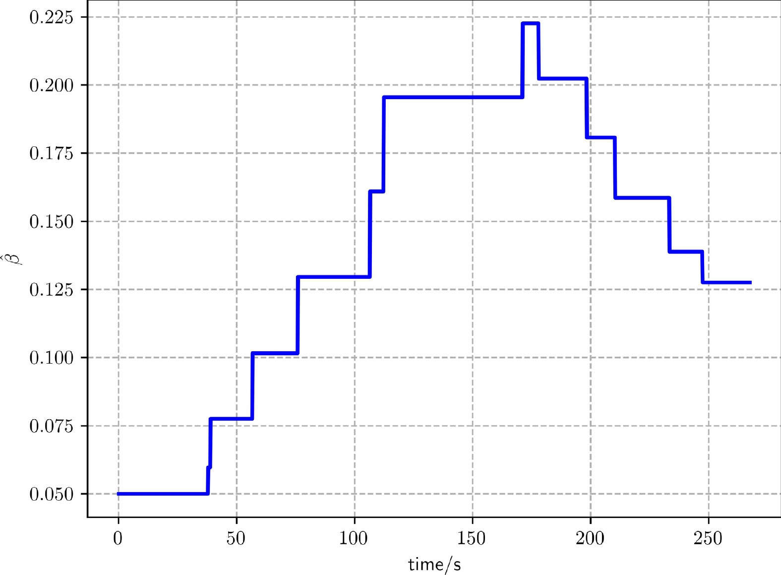
Figure 5.
The curve of the estimate of the target behavior parameter throughout the tracking process in Fig. 4.
-
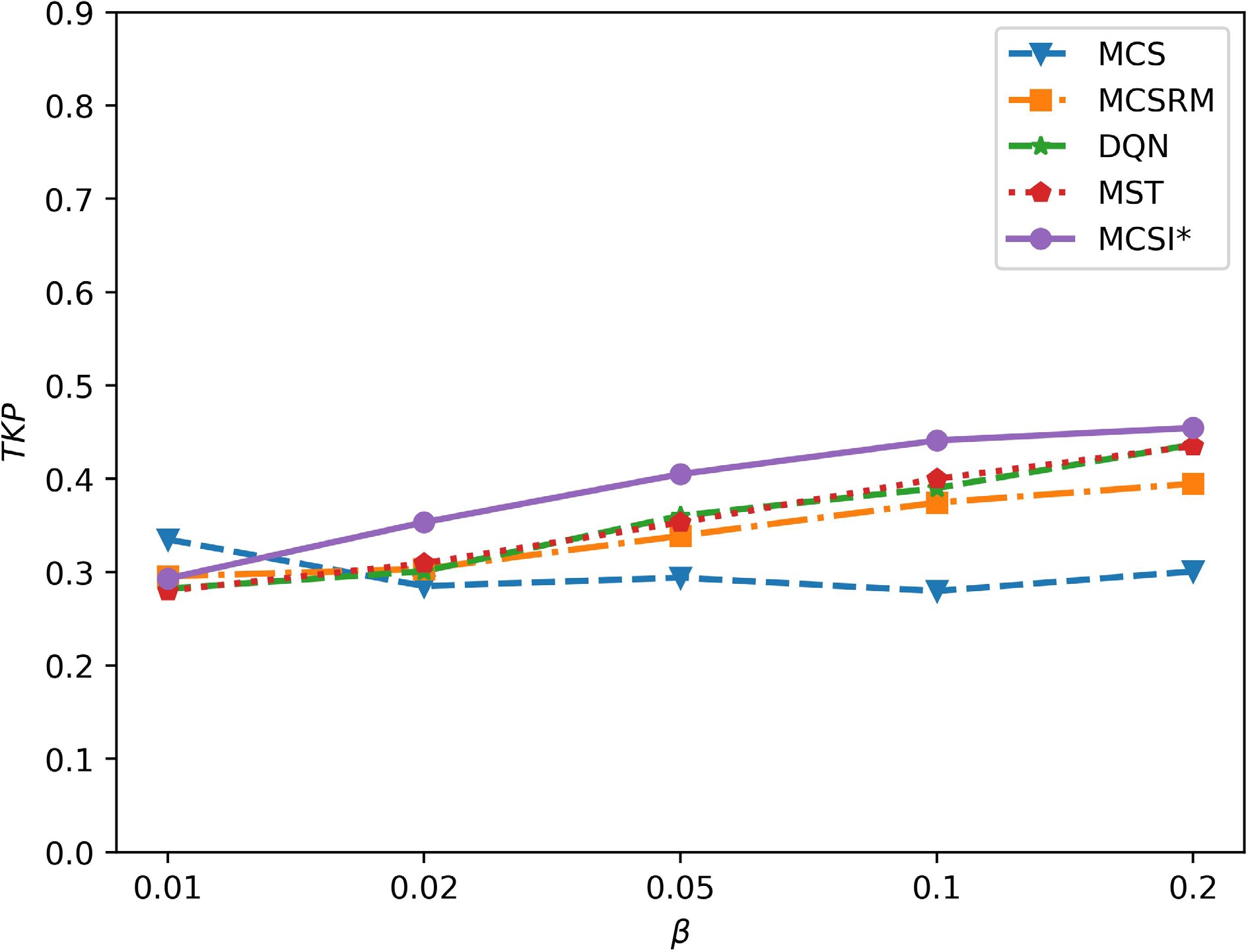
Figure 6.
The impacts of the target's global motion behavior on tracking performance.
-
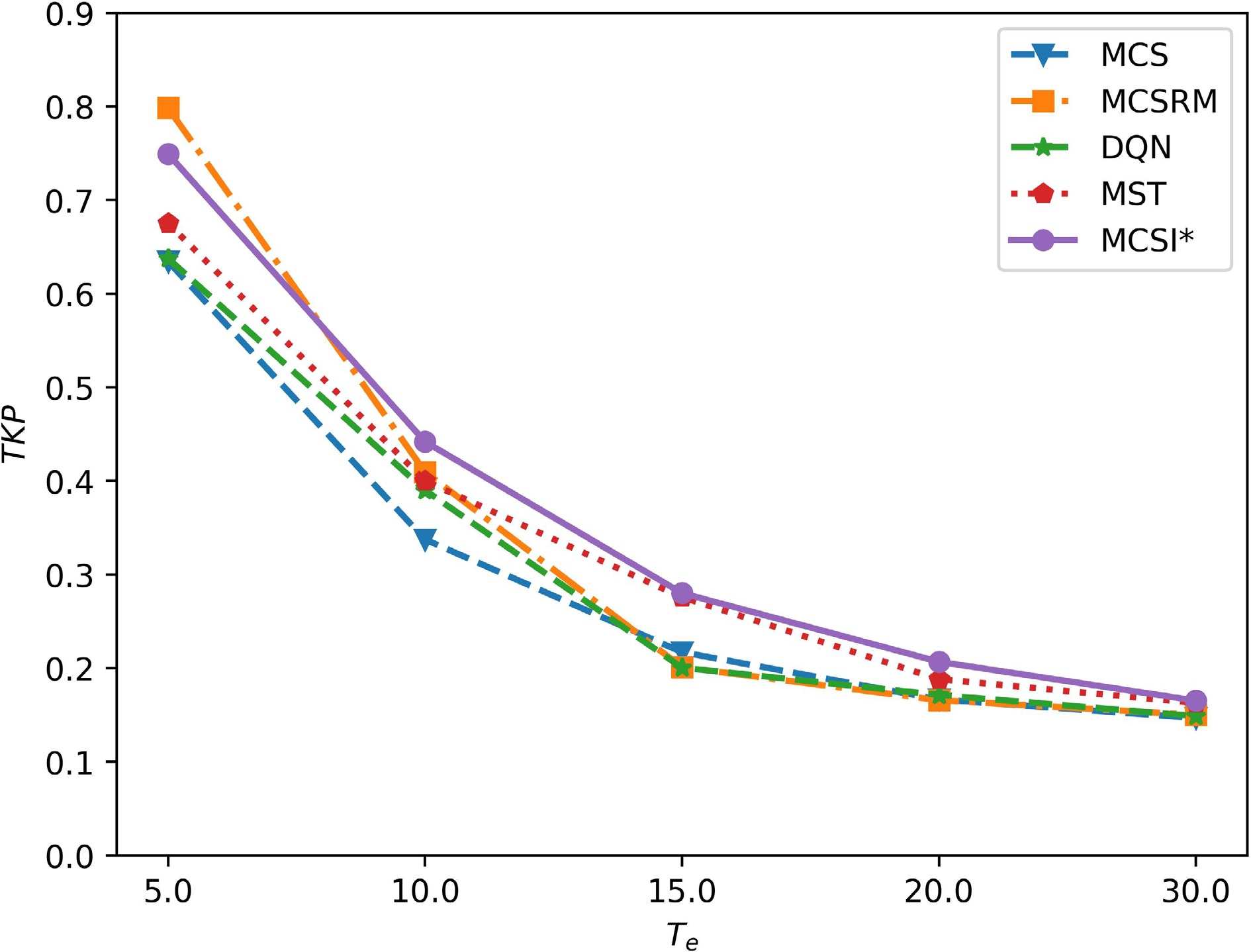
Figure 7.
The impacts of the target's evasive behavior on tracking performance.
-
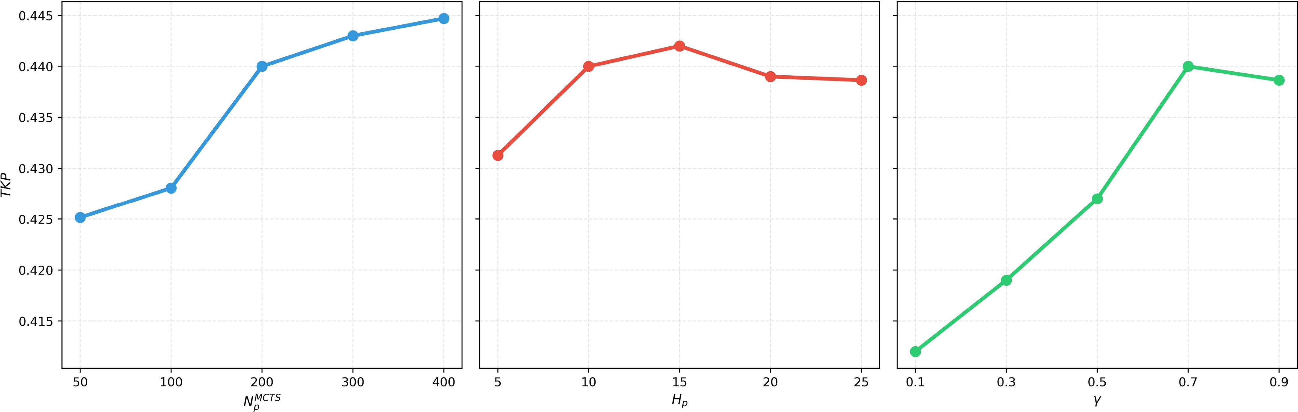
Figure 8.
The impacts of the key parameters on tracking performance.
-
Input: Urban road graph $ M=(V,E) $ $ {g}_{i}({g}_{i}\in \mathbf{g}) $ $ C $ $ x_{T}^{t} $ $ x_{U}^{t} $ $ N_{T}^{MC} $ Output: The probability $ P(E({v}_{i},{v}_{j},{t}_{1},{t}_{2})) $ 1: //The target does not reach its goal region 2: while $ x_{T}^{t} $ $ {g}_{T} $ 3: //Target is in the UAV's FOV or in the sensing field of ground sensors 4: if $ x_{T}^{t}\in {F}_{t} $ $ x_{T}^{t}\in {S}_{c} $ 5: //Update target's intention 6: $ P({g}_{T}|x_{T}^{0: t})\propto P(v_{T}^{n}|v_{T}^{c},{g}_{T},\Omega )P({g}_{T}|x_{T}^{0: t-1}) $ 7: // Sampled trajectories 8: $ \Theta \leftarrow \varnothing $ 9: for each $ {g}_{i}\in \mathbf{g} $ 10: // Calculate the number of trajectories 11: $ N_{i}^{MC}=N_{T}^{MC}P({g}_{i}|x_{T}^{0: t}) $ 12: for $ i=1,2,...,N_{i}^{MC} $ 13: Draw a sample trajectory ${\mathcal{T}}$ $ v_{T}^{l} $ $ {g}_{i} $ 14: $\Theta \leftarrow \Theta \cup {\mathcal{T}}$ 15: end for 16: end for 17: for each ${\mathcal{T}} \in \Theta $ 18: // $ {v}_{j} $ $ {v}_{i} $ ${\mathcal{T}}$ 19: for each $({v_i},{v_j}) \in {\mathcal{T}}$ 20: Record the times $ {t}_{T}({v}_{i}) $ $ {t}_{T}({v}_{j}) $ 21: end for 22: end for 23: end if 24: Calculate $ P(E({v}_{i},{v}_{j},{t}_{1},{t}_{2})) $ 25: end while Table 1.
Target trajectory prediction algorithm (MCSI)
-
Input: Urban road graph $ M=(V,E) $ $ {g}_{i}({g}_{i}\in \mathbf{g}) $ $ P({g}_{i}|x_{T}^{0: t}) $ $ x_{T}^{t} $ $ x_{U}^{t} $ $ N_{p}^{MCTS} $ $ {H}_{p} $ $\lambda $ Output: The next goal node of the UAV, $ v_{U}^{*}(t+1) $ 1: //Target is not in the UAV's FOV 2: if $ x_{T}^{t}\notin {F}_{t} $ 3: Create root node $ {v}_{0} $ $ v_{U}^{n}(t) $ 4: for $ i=1,2,... $ $ N_{p}^{MCTS} $ 5: $ {v}_{l}\leftarrow $ $ ({v}_{0}) $ 6: $ {r}_{l}\leftarrow $ $ ({v}_{l}) $ 7: BACKUP $ ({v}_{l},{r}_{l}) $ 8: end for 9: $ v_{U}^{*}(t+1)\leftarrow $ $ ({v}_{0},0) $ 10: end if 11: function TREEPOLICY(v) 12: while v is a nonterminating state do 13: if v is not fully expanded then 14: return EXPAND(v) 15: else 16: v←BESTCHILD(v, $ \lambda $ 17: end if 18: end while 19: return v 20: end function 21: function EXPAND(v) 22: Choose one of the unvisited child nodes $ {\overline{v}}_{i} $ $ {\overline{v}}_{i}\in \chi (v) $ 23: return $ {\overline{v}}_{i} $ 24: end function 25: function BESTCHILD(v, $ \lambda $ 26: return $ \underset{{v}_{i}\in \chi (v)}{\arg \max }\dfrac{Q({v}_{i})}{N({v}_{i})}+\lambda \sqrt{\dfrac{\log (N(v))}{N({v}_{i})}} $ 27: end function 28: function DEFAULTPOLICY( $ (v_{U}^{n}(t+k)) $ 29: Randomly sampling a goal region $ {g}_{i} $ $ P({g}_{i}|x_{T}^{0: t}) $ 30: Draw a sample trajectory $ {\mathcal{T}} $ $ v_{U}^{n}(t+k) $ $ {g}_{i} $ $ V_{\max }^{U} $ 31: $ \begin{aligned}r\leftarrow \sum \limits_{i=0}^{{H}_{p}-1}{\gamma }^{i}P(E(v_{U}^{n}(t+i),v_{U}^{n}(t+i+1), {t}_{U}(v_{U}^{n}(t+i)),{t}_{U}(v_{U}^{n}(t+i+1)))) \end{aligned} $ 32: return r 33: end function 34: function BACKUP(v, r) 35: while v is not None do 36: $ N(v)\leftarrow N(v)+1 $ 37: $ Q(v)\leftarrow Q(v)+r $ 38: $ v\leftarrow $ $ v $ 39: end while 40: end function Table 2.
MCTS-based planning method.
-
Statistical
indicatorsMean Standard
deviationU-statistic One-sided
p-valueMCS 0.32 0.15 6,912 0.000002 MCSRM 0.38 0.17 6,158 0.002340 DQN 0.39 0.18 5,927 0.011790 MST 0.40 0.17 5,678 0.048912 MCSI* 0.44 0.18 5,000 0.500488 Table 1.
Statistical significance results.
Figures
(8)
Tables
(3)