-
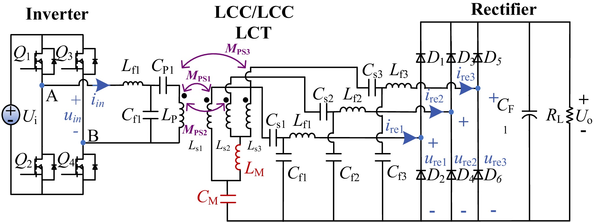
Figure 1.
The circuit diagram of a WPT system with decoupling DDQ coils.
-
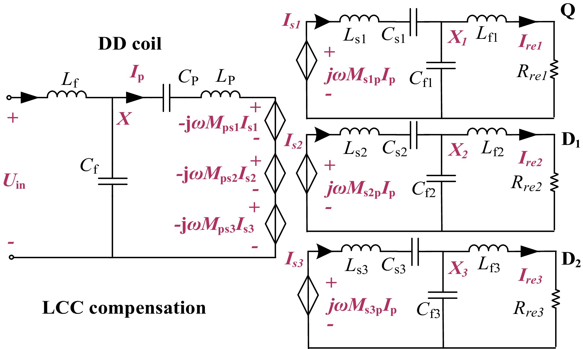
Figure 2.
The controlled source equivalent model diagram.
-
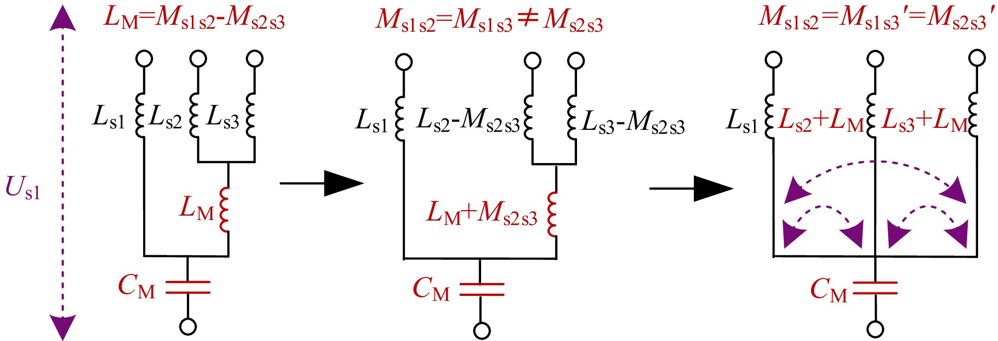
Figure 3.
Decoupling model of a DDQ coil.
-
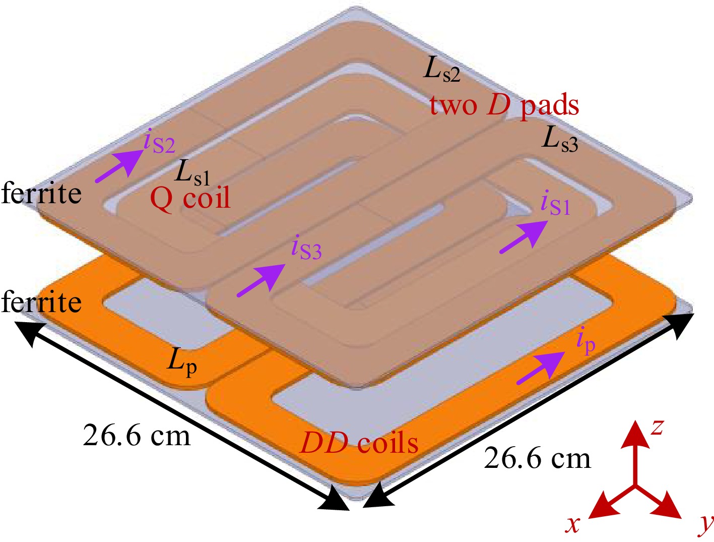
Figure 4.
Schematic diagram of a decoupling DDQ coil.
-
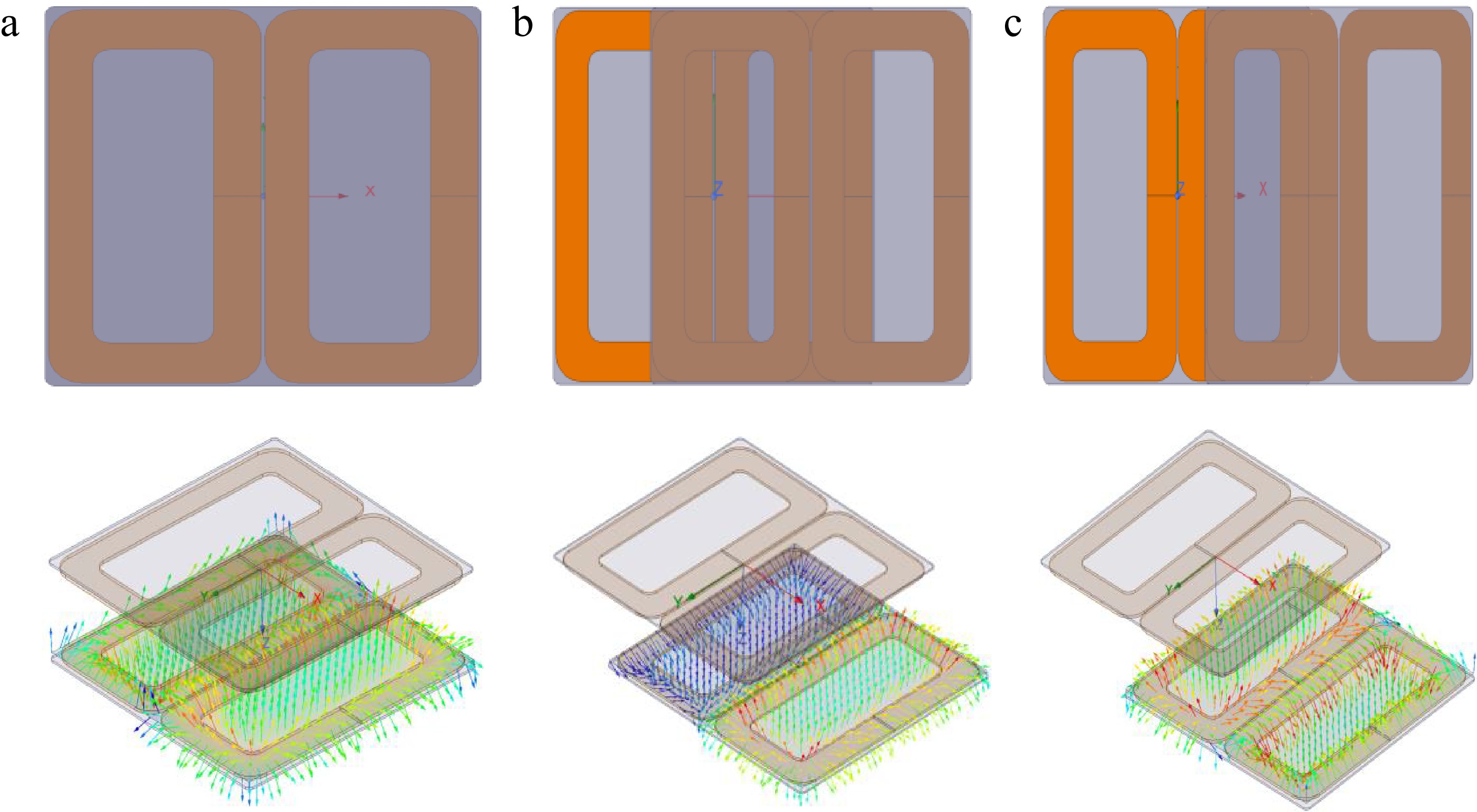
Figure 5.
The relative position diagram when both the primary and secondary sides are DD coils and the schematic diagram of the secondary side receiving magnetic induction lines: (a) facing position, (b) misaligned 8 cm along the Y direction, (c) misaligned 12 cm along the Y direction.
-
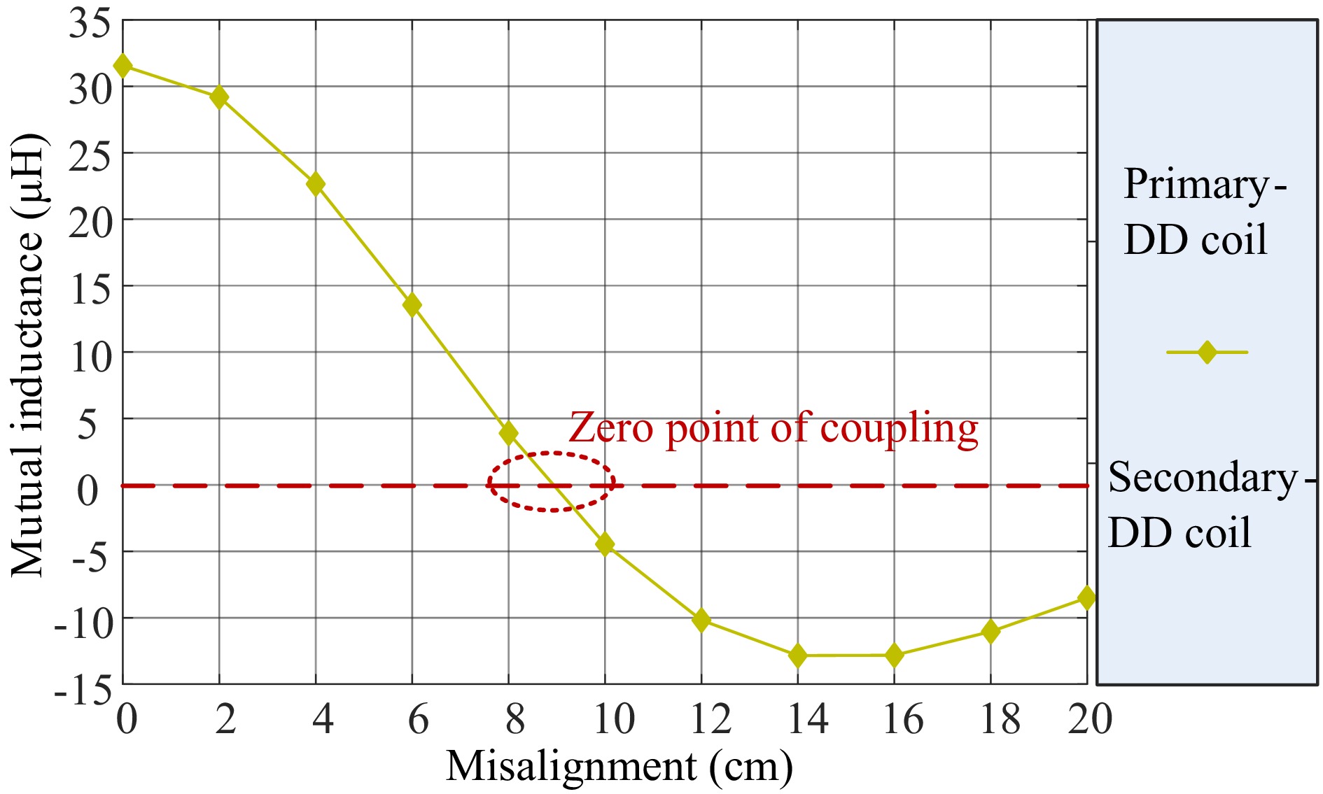
Figure 6.
Mutual inductance curve of the DD coil misaligned along the Y direction.
-
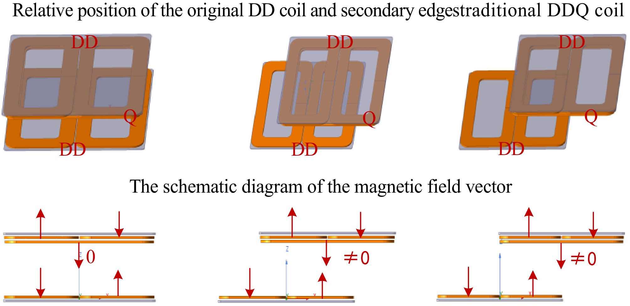
Figure 7.
The schematic and position diagram of the magnetic field vector when the primary side is the DD coil and the secondary side is the DDQ coil displaced along the Y direction.
-
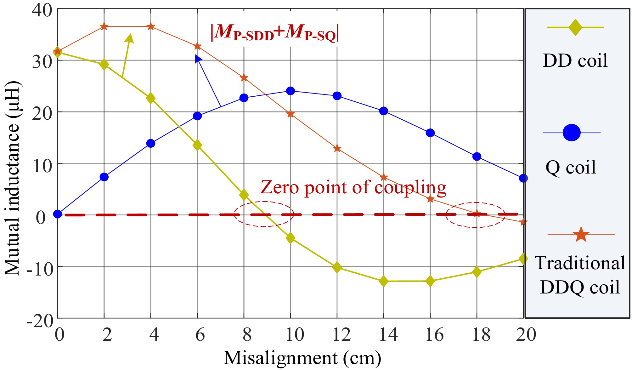
Figure 8.
Mutual inductance curve of the DDQ coil misaligned along the Y direction.
-
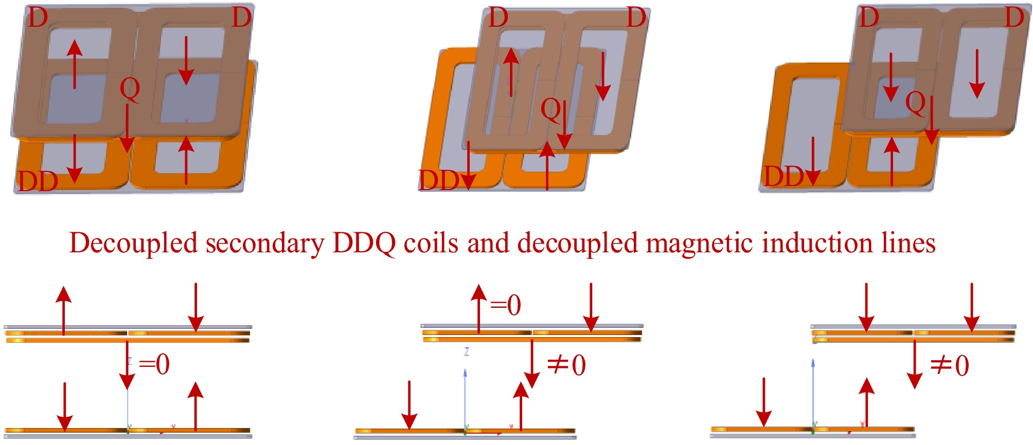
Figure 9.
Schematic diagram of magnetic induction lines with mutual decoupling DDQ coils displaced along the Y direction.
-
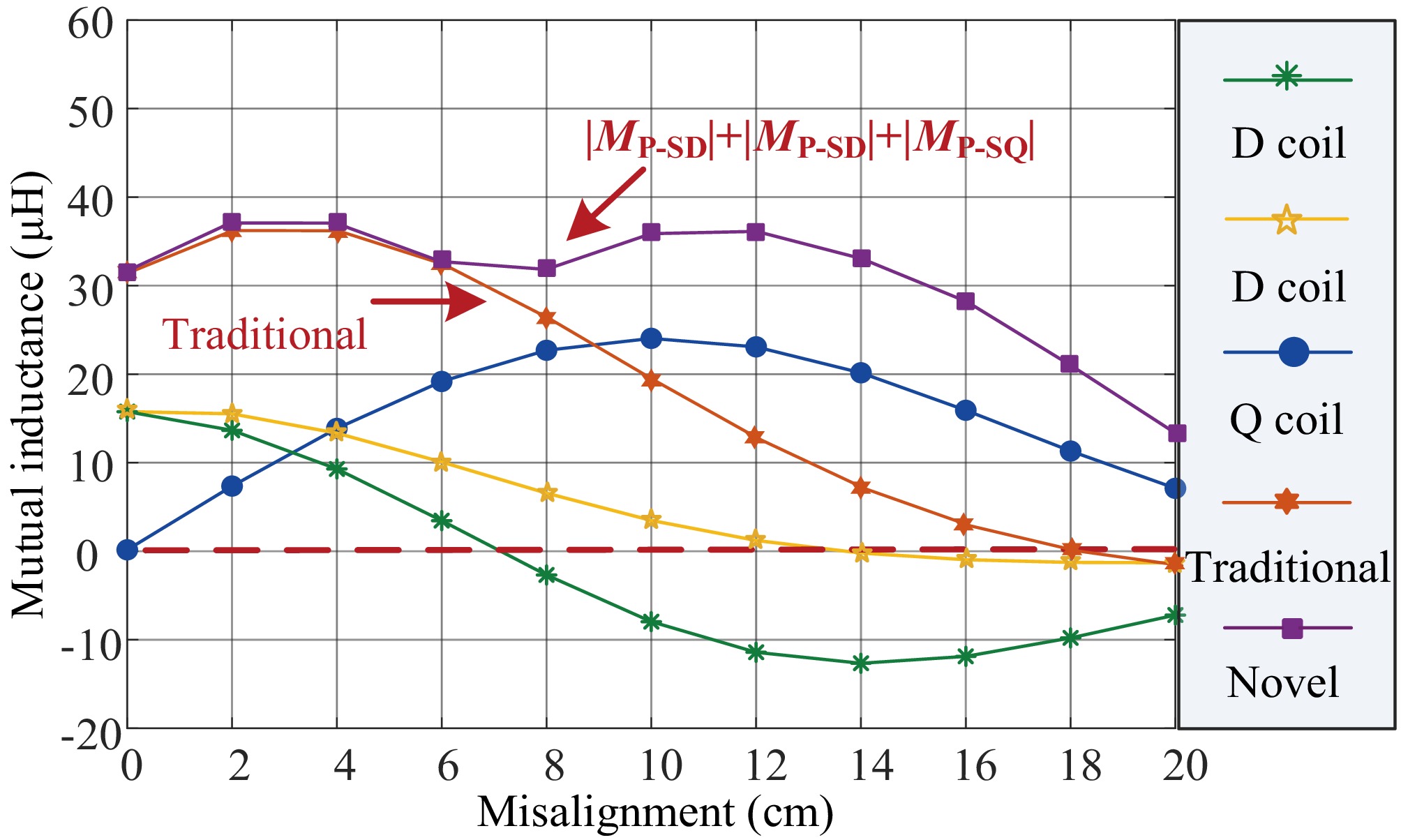
Figure 10.
Curve of mutual inductance between a decoupling DDQ coil and a primary coil with Y-axis misalignment.
-
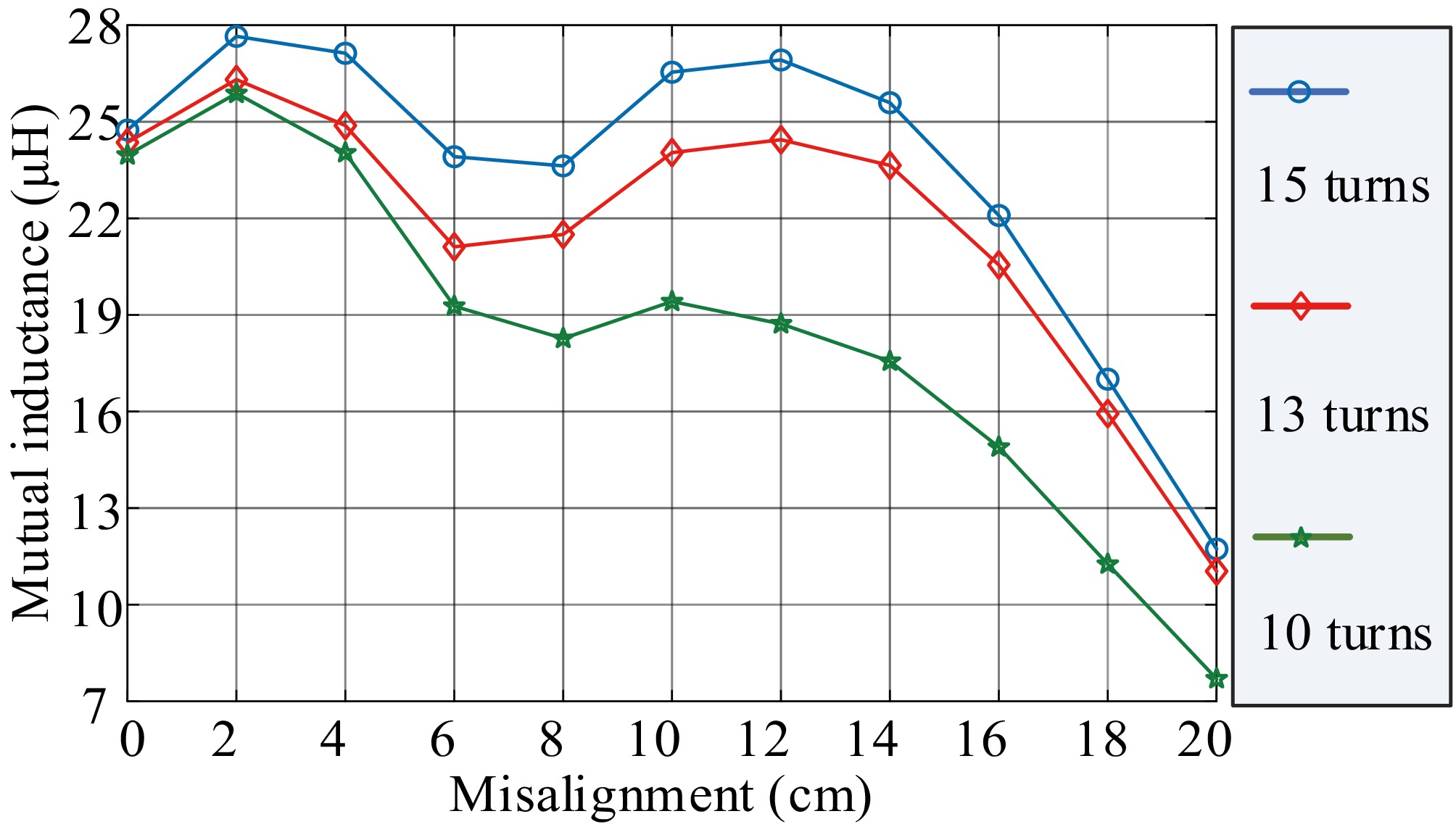
Figure 11.
Equivalent mutual inductance of magnetic coupling structure under different turns of the Q coil.
-
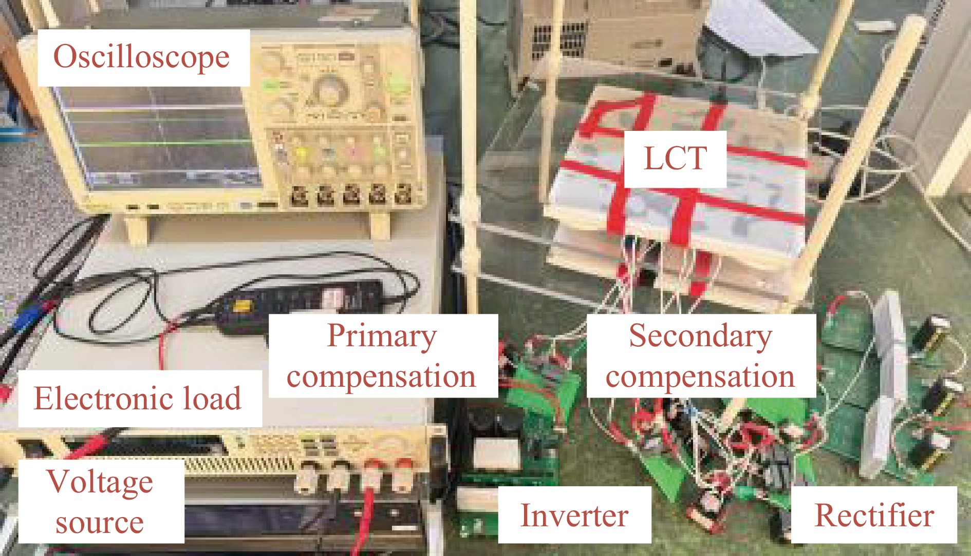
Figure 12.
The experimental prototype.
-
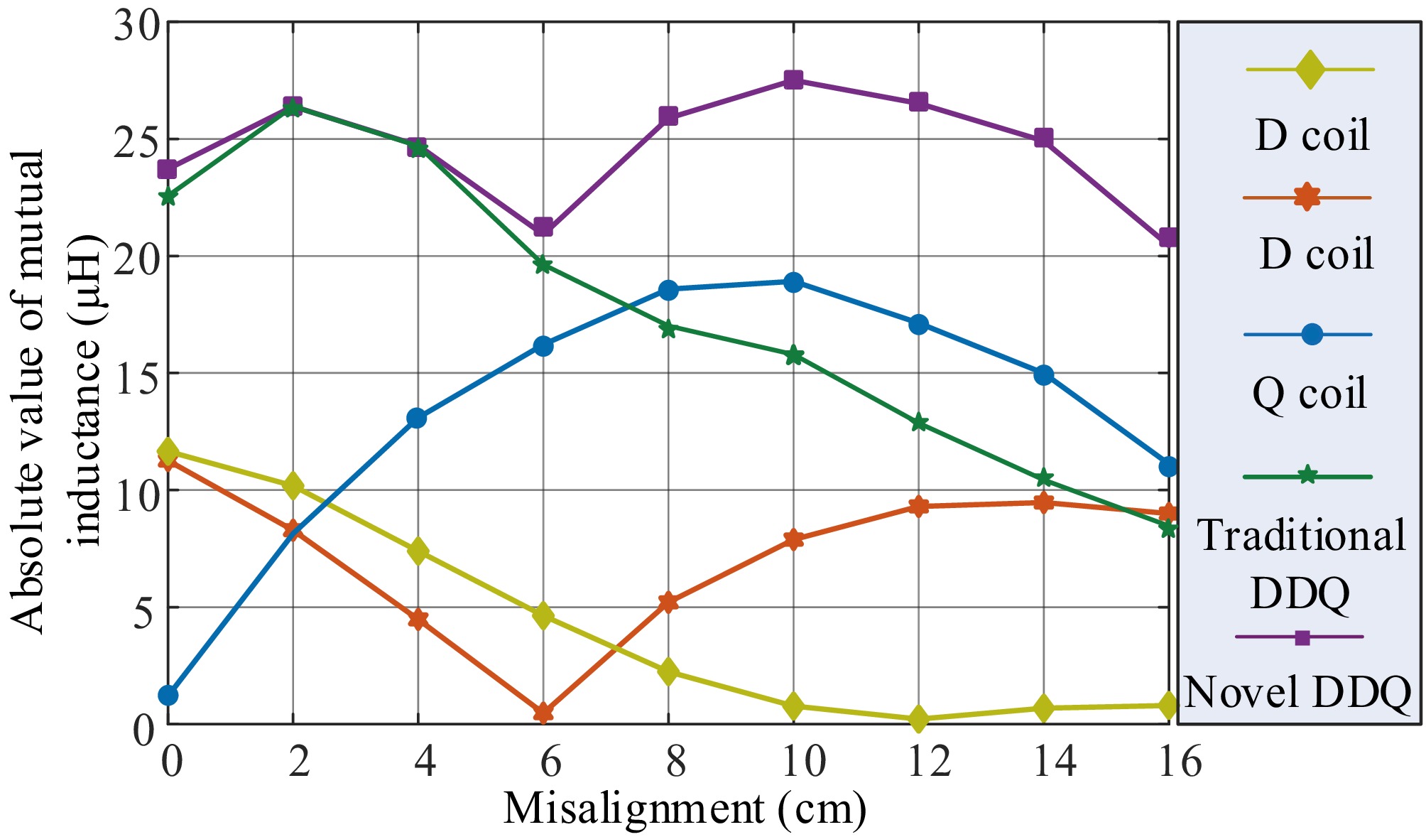
Figure 13.
Actual measurement of coil mutual inductance.
-
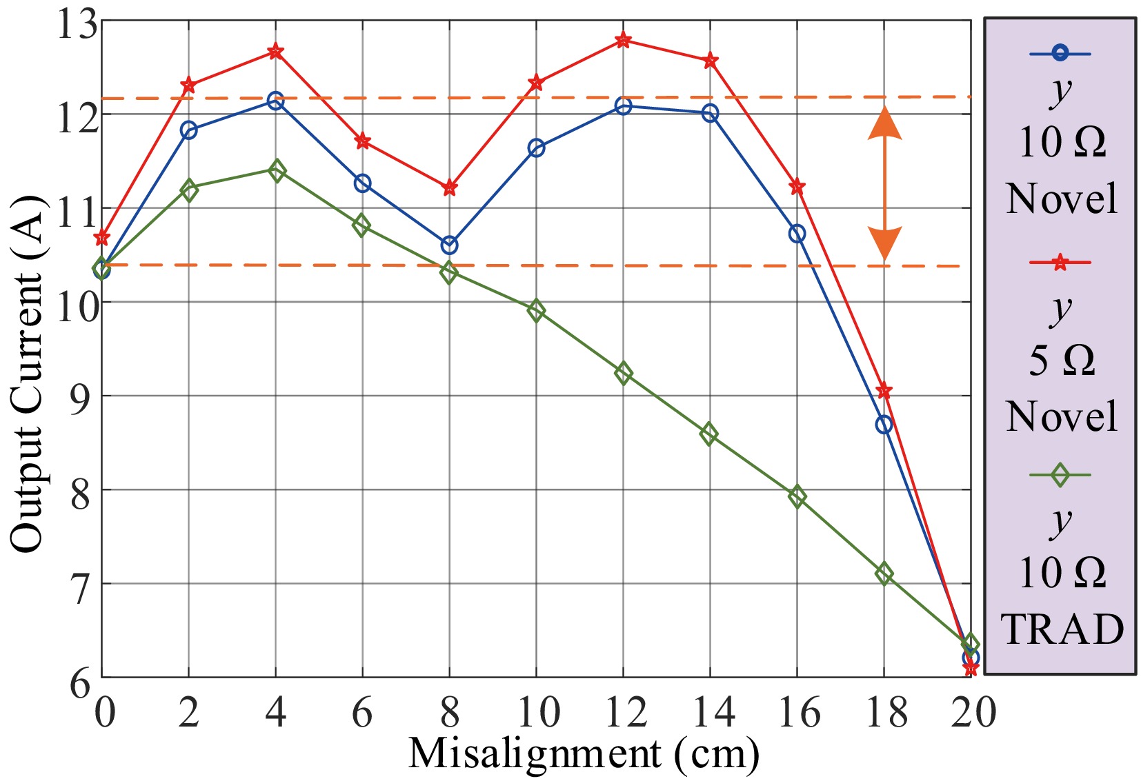
Figure 14.
The curves of output current with coil misalignment.
-
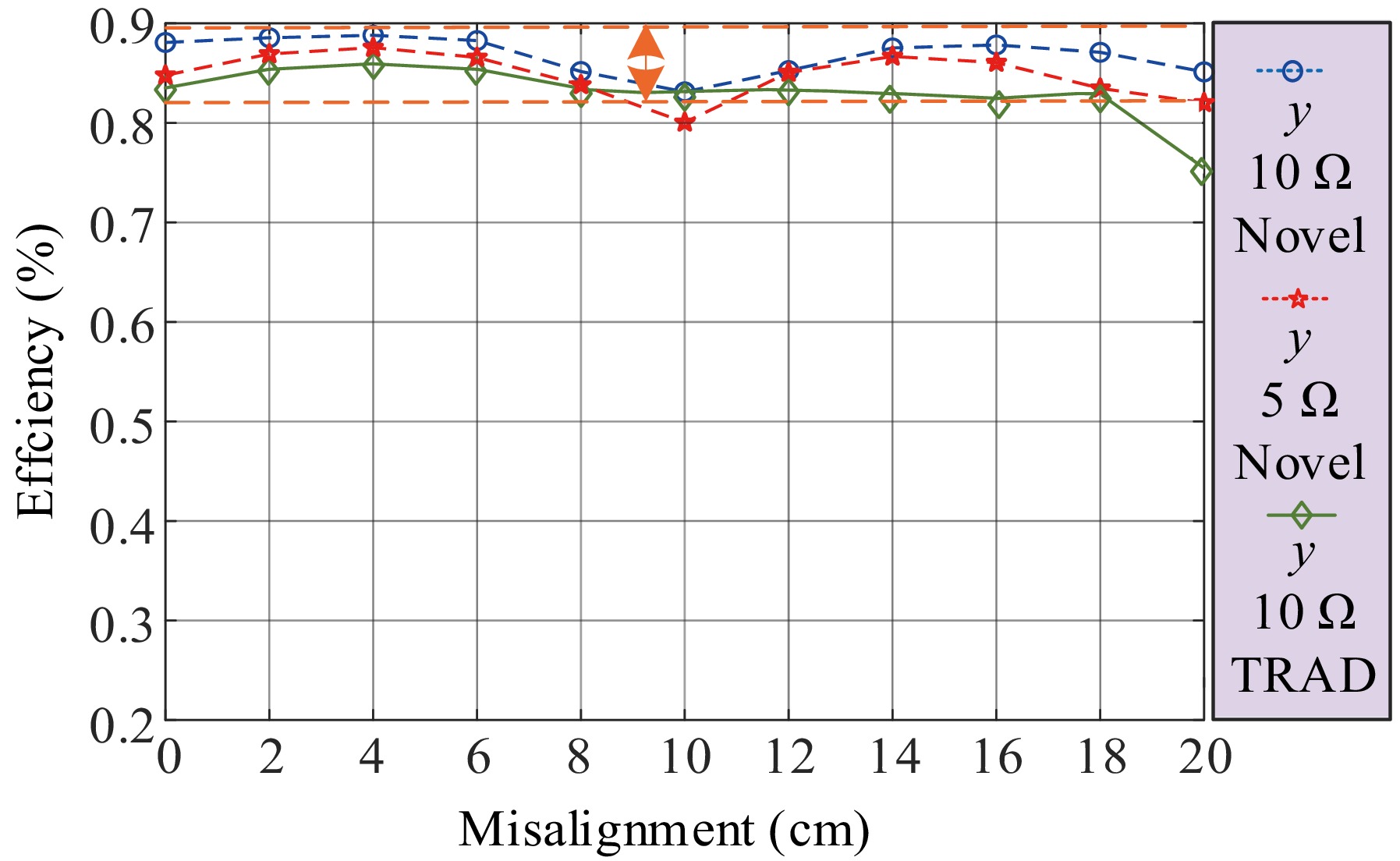
Figure 15.
The curves of efficiency with coil misalignment.
-
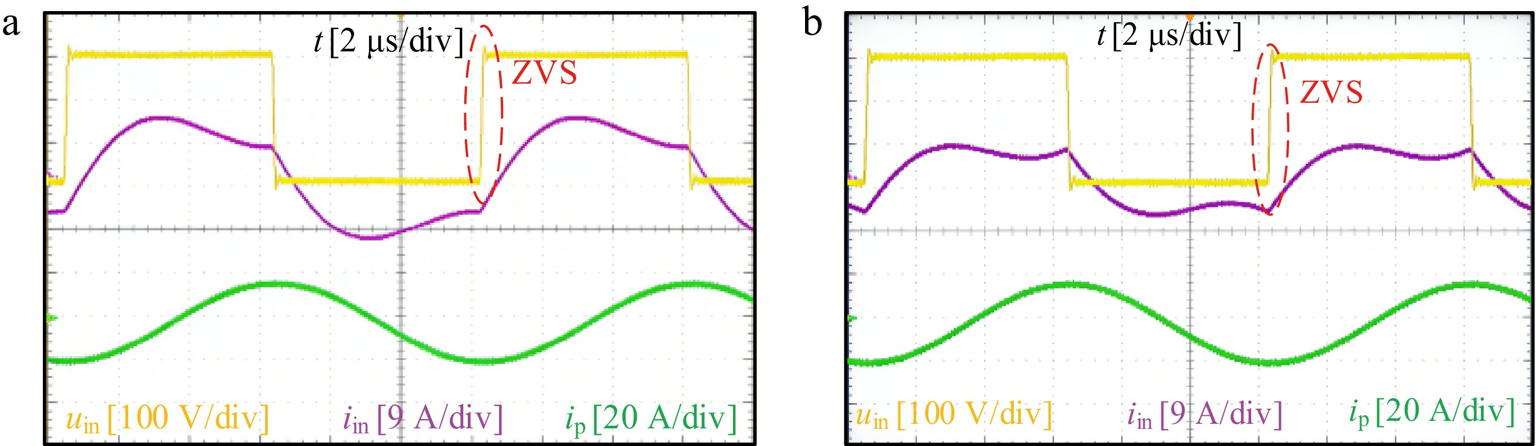
Figure 16.
Experimental waveforms of inverter voltage, current, and coil current at the facing position. (a) 10 Ω. (b) 5 Ω.
-
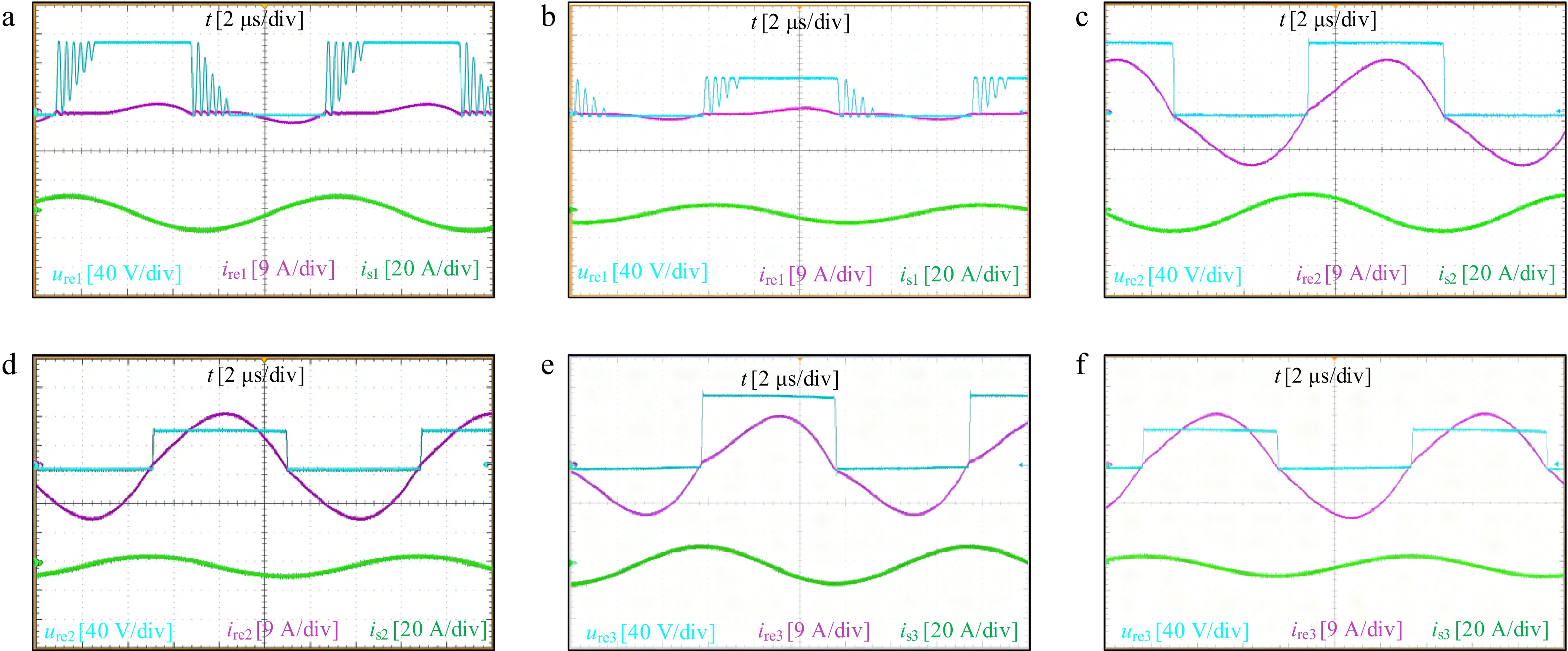
Figure 17.
Experimental waveforms of rectifier voltage, current, and coil current in the facing position. (a) Secondary-side Q coil, 10 Ω. (b) Secondary-side Q coil, 5 Ω. (c) Secondary-side D coil, 10 Ω. (d) Secondary-side D coil, 5 Ω. (e) Another secondary-side D coil, 10 Ω. (f) Another secondary-side D coil, 5 Ω.
-
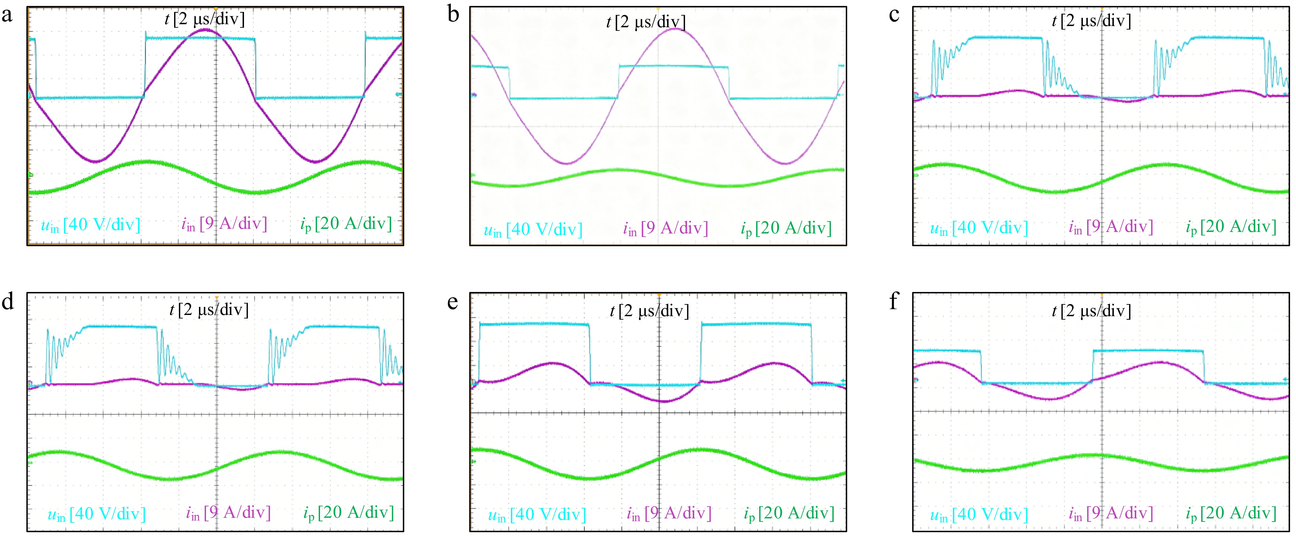
Figure 18.
Experimental waveforms of rectifier voltage, current, and coil current with a misalignment position of 8 cm in the Y direction. (a) Secondary-side Q coil, 10 Ω. (b) Secondary-side Q coil, 5 Ω. (c) Secondary-side D coil, 10 Ω. (d) Secondary-side D coil, 5 Ω. (e) Another secondary-side D coil, 10 Ω. (f) Another secondary-side D coil, 5 Ω.
-
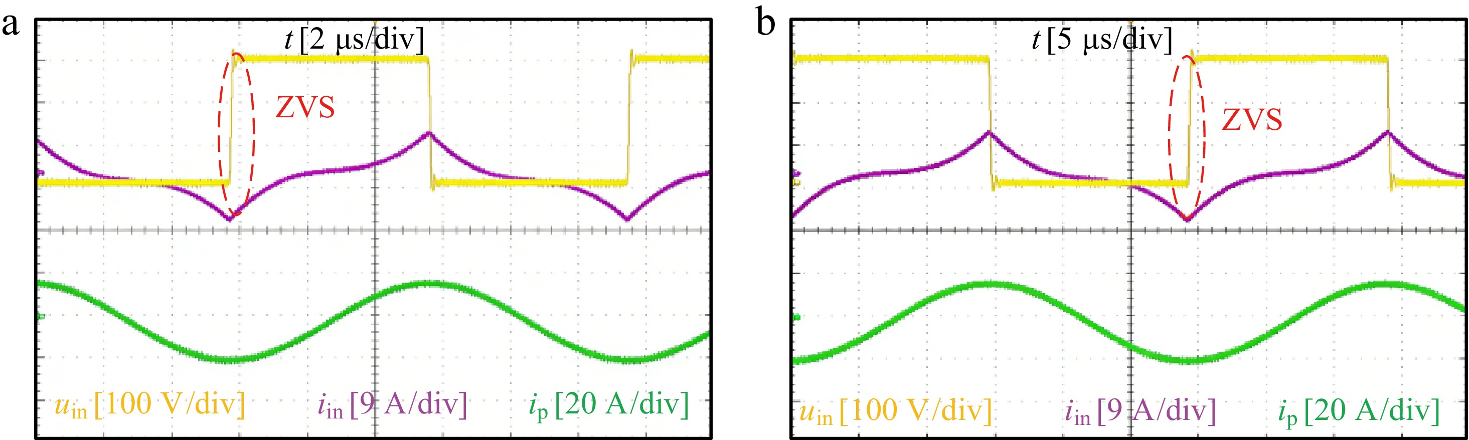
Figure 19.
Experimental waveforms of inverter voltage, current, and coil current with a misalignment position of 8 cm in the Y direction. (a) 10 Ω. (b) 5 Ω.
-
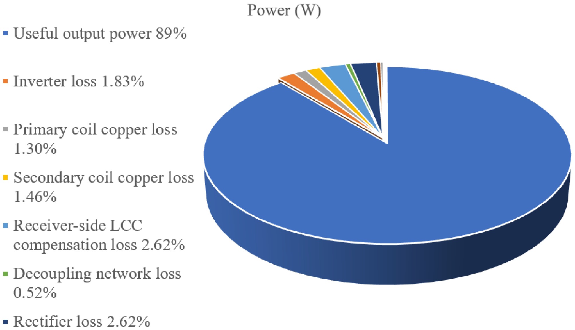
Figure 20.
The specific loss analysis diagram.
-
Parameters Value Parameters Value Ui 300.00 V f 85 kHz LP 83.41 μH MPS1 −0.55 μH LS1 124.85 μH MPS2 −11.21 μH LS2 40.69 μH MPS3 10.97 μH LS3 40.15 μH MS1S2 34.34 μH CP1 55.29 nF MS1S3 32.29 μH Cf 175.3 nF MS2S3 −5.47 μH CS1 43.93 nF Cf1, Cf2, Cf3 327.66 nF CS2 98.86 nF Lf1, Lf2, Lf3 10.00 μH CS3 100.41 nF LM 40.00 μH Lf 20.00 μH CM 102.10 nF Table 1.
The circuit parameters
-
Technology Power Cost and complexity Misalignment range and Output fluctuation Efficiency Hybrid topology[20] 3.5 kW High 0−150 mm (37.5%)
230−250 V (8%)93.96% Quadrupole receiving coils[21] 1.1 kW High 0−150 mm (50%)
60−150 V (60%)89% Reconfigurable rectifier-based IPT receivers[22] 400 W High Coupling variation k (0.1−0.4)
383.3−397.8 W (4%)94.3% This work 1.7 kW Low 0−160 mm (60%)
10.4−12 A (13.3%)89% Table 2.
Normalized and qualitative comparison with related WPT methods.
Figures
(20)
Tables
(2)