-
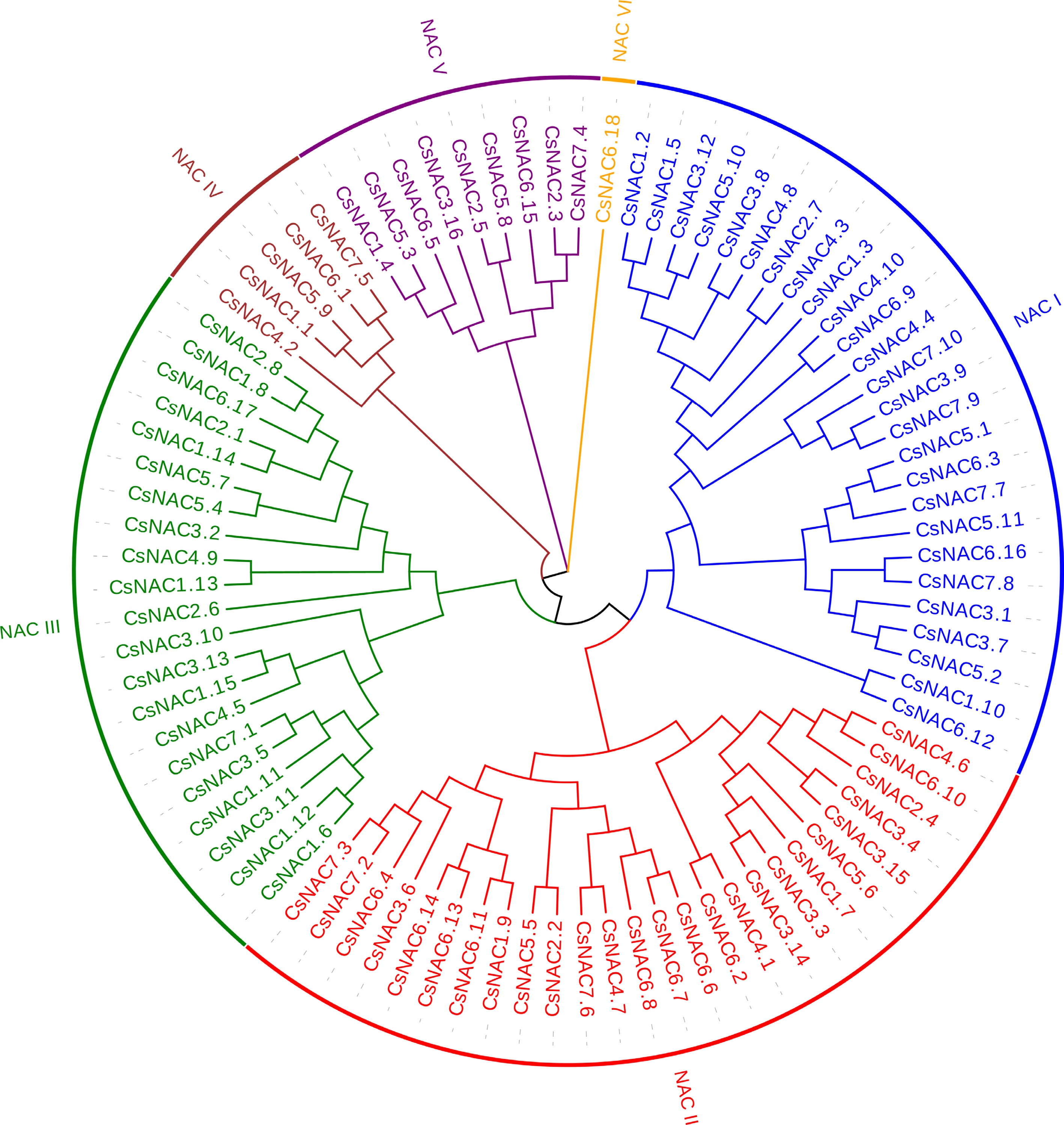
Figure 1.
Phylogenetic tree of NAC proteins in cucumber. Amino acid sequences were aligned using CLUSTAL W, and a phylogenetic tree with 1,000 bootstrap replicates was generated using MEGA 11. Each subfamily is distinctly represented by a specific color.
-
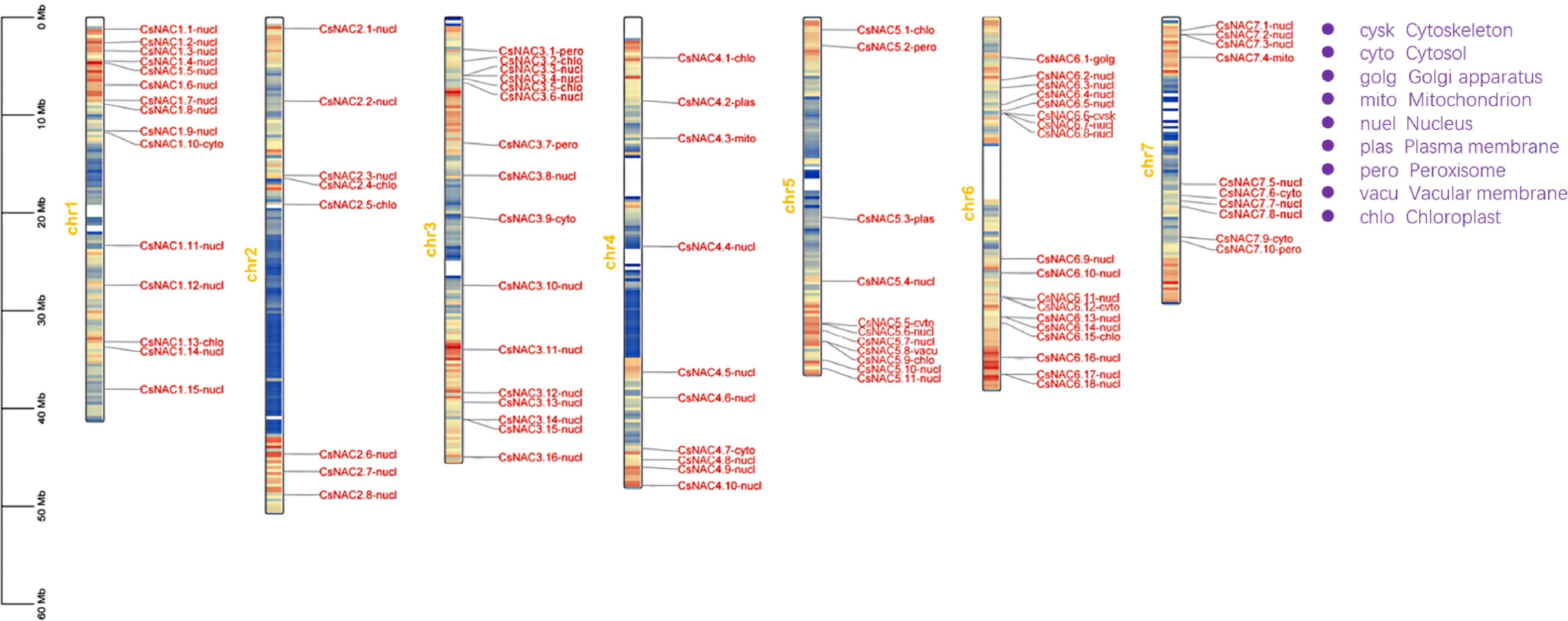
Figure 2.
Chromosomal localization and subcellular localization prediction of the cucumber NAC gene family. The left scale indicates chromosome length, with gene names followed by their predicted subcellular localizations. Full names are labeled in purple at the top right. Yellow numbers indicate chromosome counts, and the blue-to-red gradient represents gene density.
-
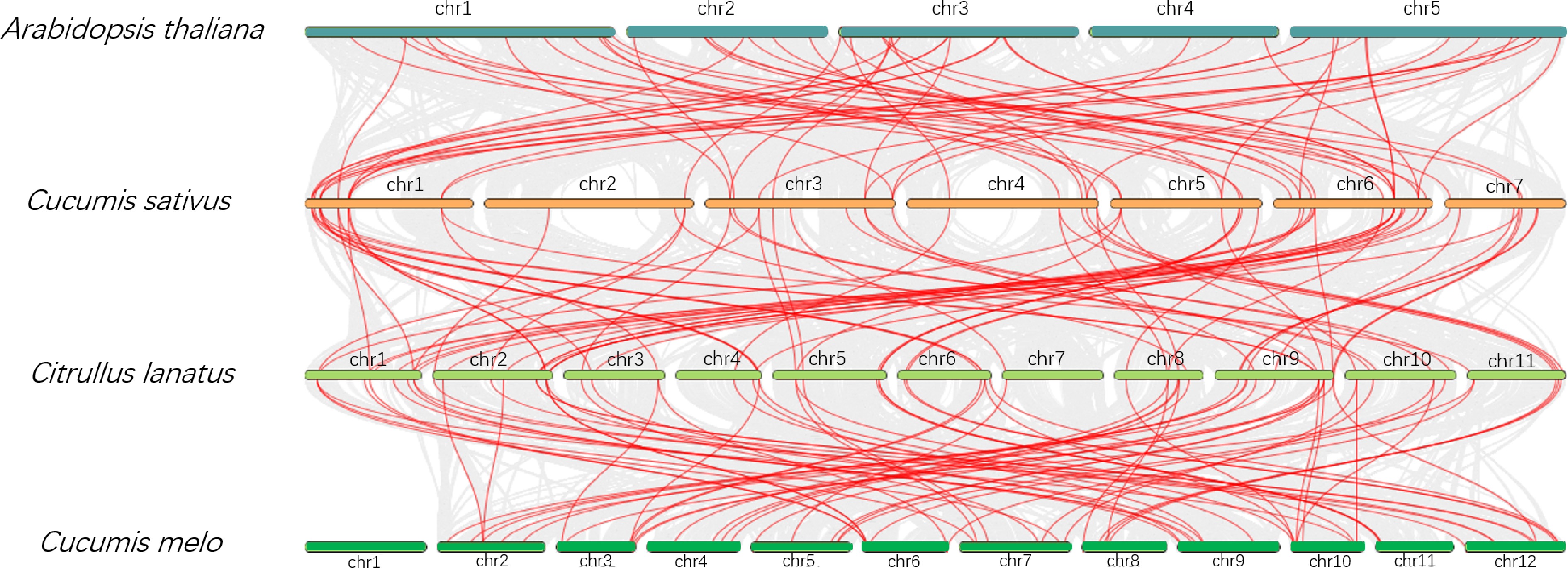
Figure 3.
Comparative analysis of NAC gene family collinearity among cucumber, watermelon, melon, and Arabidopsis. Chromosomes are color-coded by species, and chromosome numbers are labeled. Gene locations are linked across species with red lines.
-
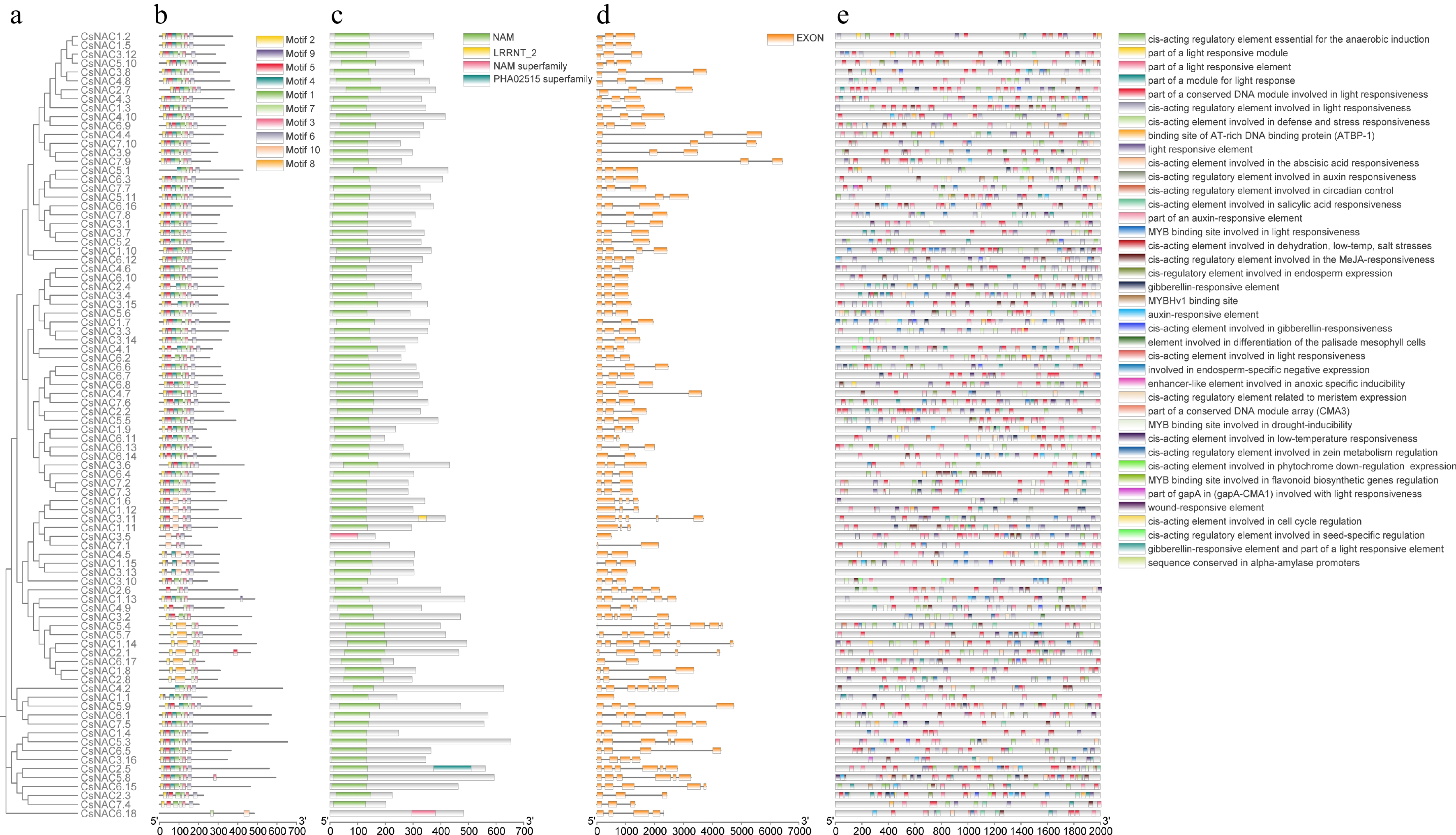
Figure 4.
Phylogenetic, exon-intron structure, and cis-element analysis of CsNAC genes. (a) Phylogenetic tree of gene family members. (b) Distribution of conserved motifs. (c) Protein structural domains. (d) Exon distribution. (e) Distribution of cis-regulatory elements in the promoter region (−2,000 bp). Different colors and shapes represent various types of cis-regulatory elements.
-
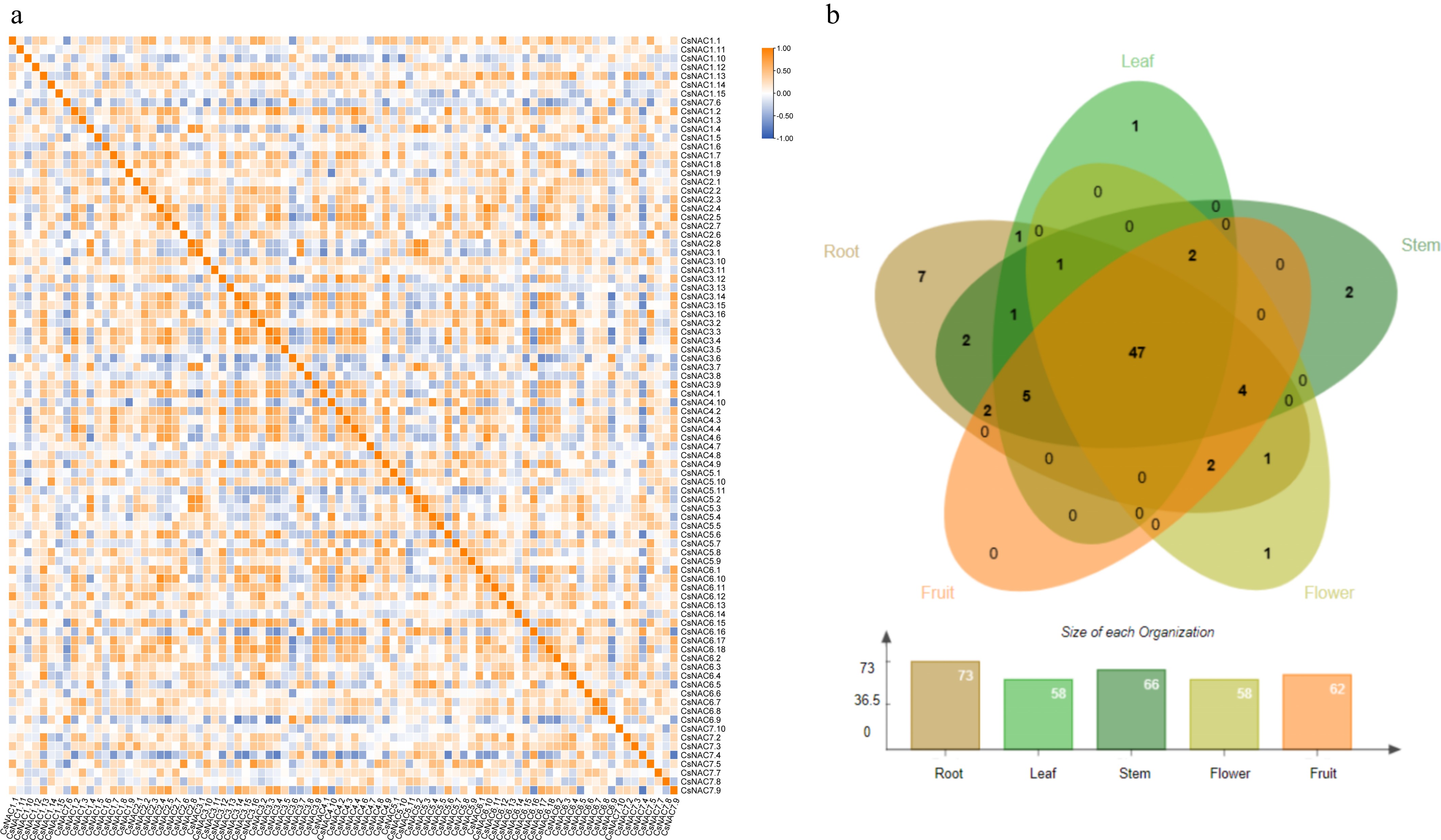
Figure 5.
Transcriptomic expression analysis of the NAC gene family. (a) Heatmap of correlation analysis of expression levels. The correlation strength is indicated by a color gradient from white to orange-yellow, with 1 representing perfect positive correlation, −1 indicating perfect negative correlation, and 0 indicating no correlation. (b) Expression of NAC genes in different tissues. Different tissues are represented by distinct colors, with a bar chart indicating the number of genes expressed in each tissue.
-
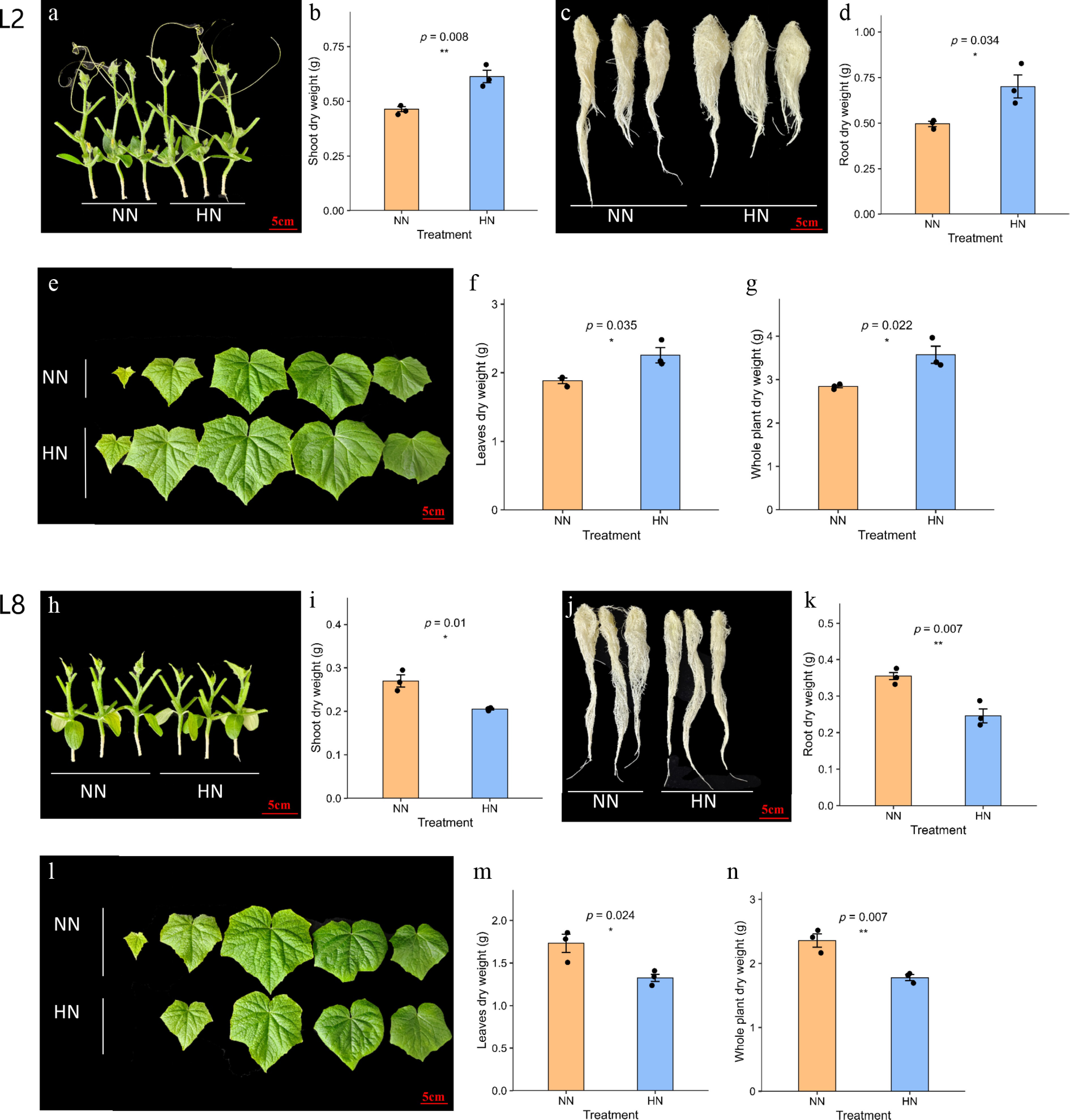
Figure 6.
Biomass responses of the high-NUE line L2 and low-NUE line L8 under NN and HN conditions. (a) Representative stem phenotype of L2; (b) stem dry weight of L2; (c) representative root phenotype of L2; (d) root dry weight of L2; (e) representative leaf phenotype of L2; (f) leaf dry weight of L2; (g) whole-plant dry weight of L2; (h) representative stem phenotype of L8; (i) stem dry weight of L8; (j) representative root phenotype of L8; (k) root dry weight of L8; (l) representative leaf phenotype of L8; (m) leaf dry weight of L8; and (n) whole-plant dry weight of L8. Data are presented as mean ± SD (n = 3). * Indicate significant differences between NN and HN treatments (* p < 0.05, ** p < 0.01; student's t-test).
-
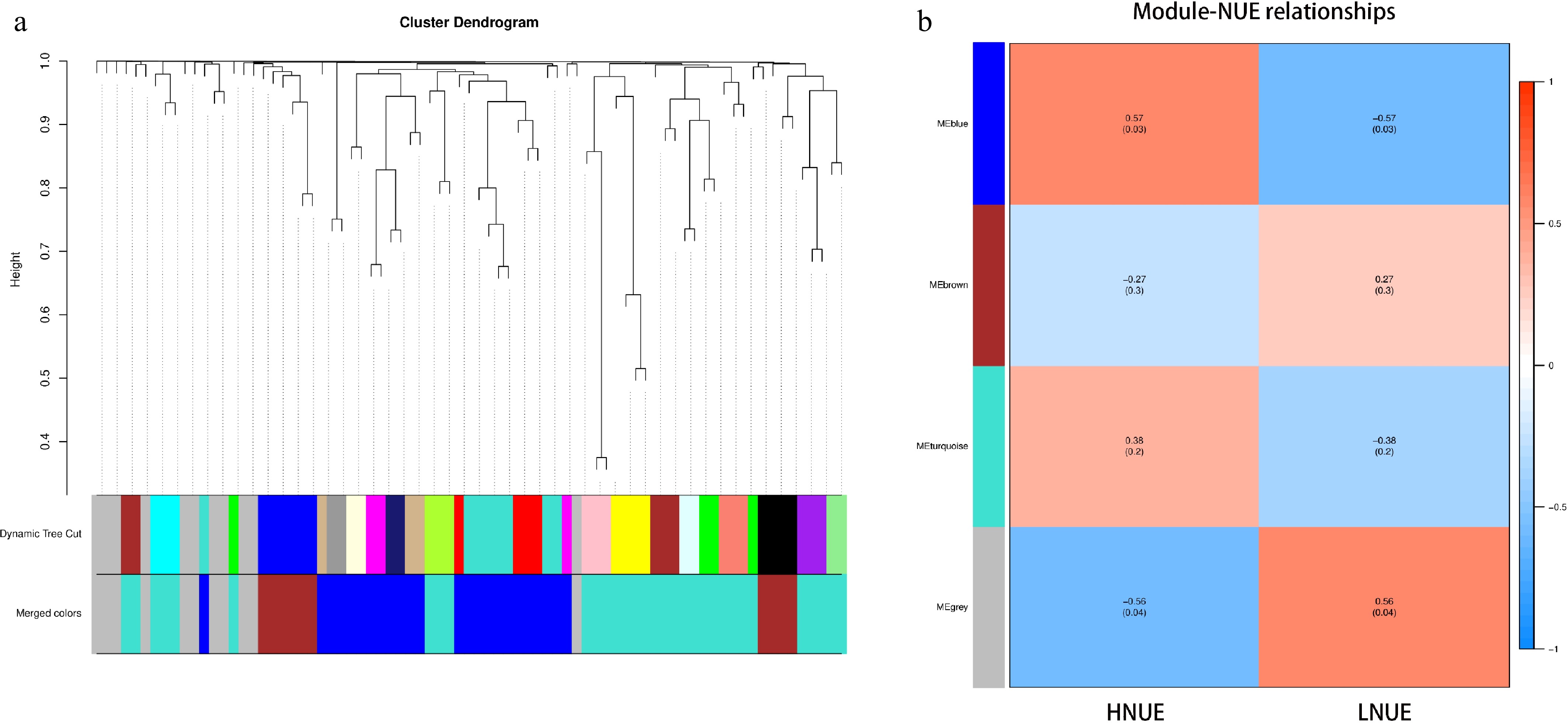
Figure 7.
The identification of key modules through WGCNA. (a) Each module is represented by a unique color, grouping genes with highly similar expression patterns. These modules are constructed based on TOM similarity, clustering genes that exhibit co-expression across various samples and conditions. The uppermost part of the figure illustrates the gene clustering tree, where each leaf represents an individual gene, and different gene modules appear as branches. The middle section displays the Dynamic Tree Cut used to identify the modules, with each color denoting a distinct module. The lower part, labeled 'Merged colors', shows the result of merging modules with a dissimilarity coefficient below 0.25, further simplifying the visualization of clustered gene groups. (b) Correlation heatmap between gene co-expression modules and NUE. Red indicates positive correlations, and blue represents negative correlations. The numbers within the cells denote Pearson correlation coefficients, with corresponding p-values shown in parentheses.
-
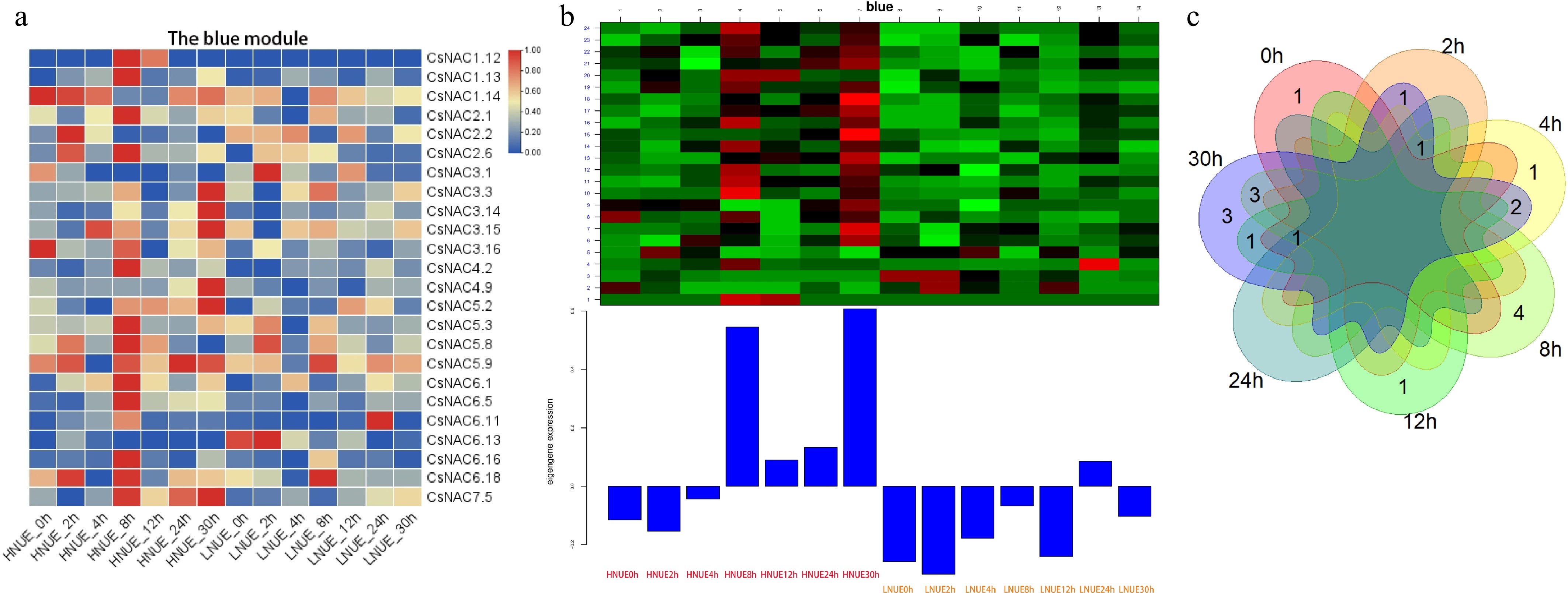
Figure 8.
Expression analysis of the module genes. (a) The expression of the genes in the blue module; (b) gene expression patterns within the blue module; (c) overlapping and unique DEGs at seven time points between high- and low-NUE lines in the blue module.
-
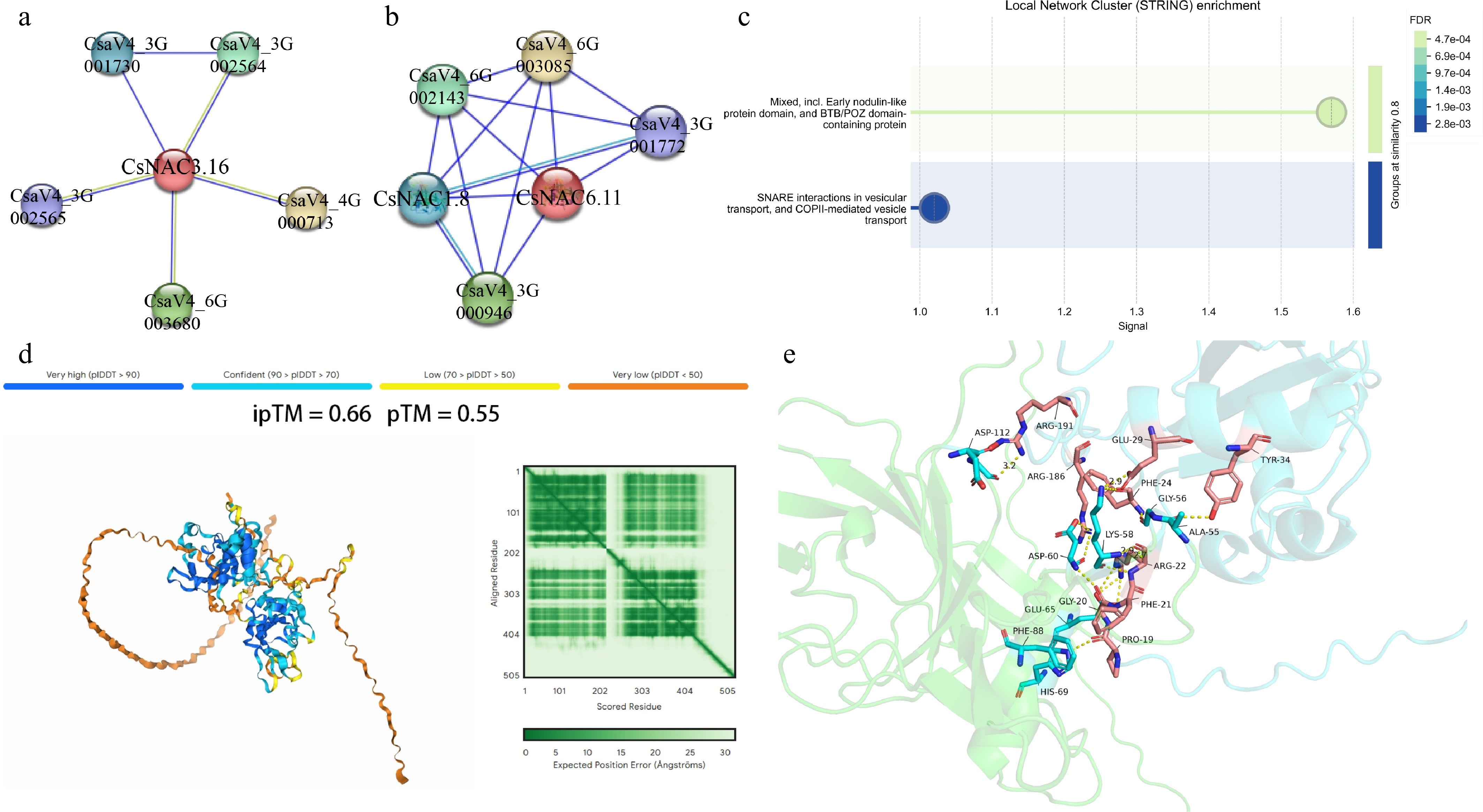
Figure 9.
Predicted protein interaction networks and structural interaction analysis of CsNAC3.16 and CsNAC6.11. (a) STRING-predicted protein interaction network of CsNAC3.16; (b) STRING-predicted protein interaction network of CsNAC6.11; (c) functional enrichment analysis of proteins predicted to interact with CsNAC3.16 and CsNAC6.11. Circle size indicates the number of genes enriched in each category, and color intensity represents the false discovery rate (FDR); (d) AlphaFold3-predicted interaction model between CsNAC6.11 and CsNAC1.8. The ipTM and pTM scores are shown as indicators of predicted interaction confidence and structural similarity; (e) predicted interaction interface between CsNAC6.11 and CsNAC1.8. Yellow dashed lines indicate potential hydrogen bonds at the predicted interaction interface.
-
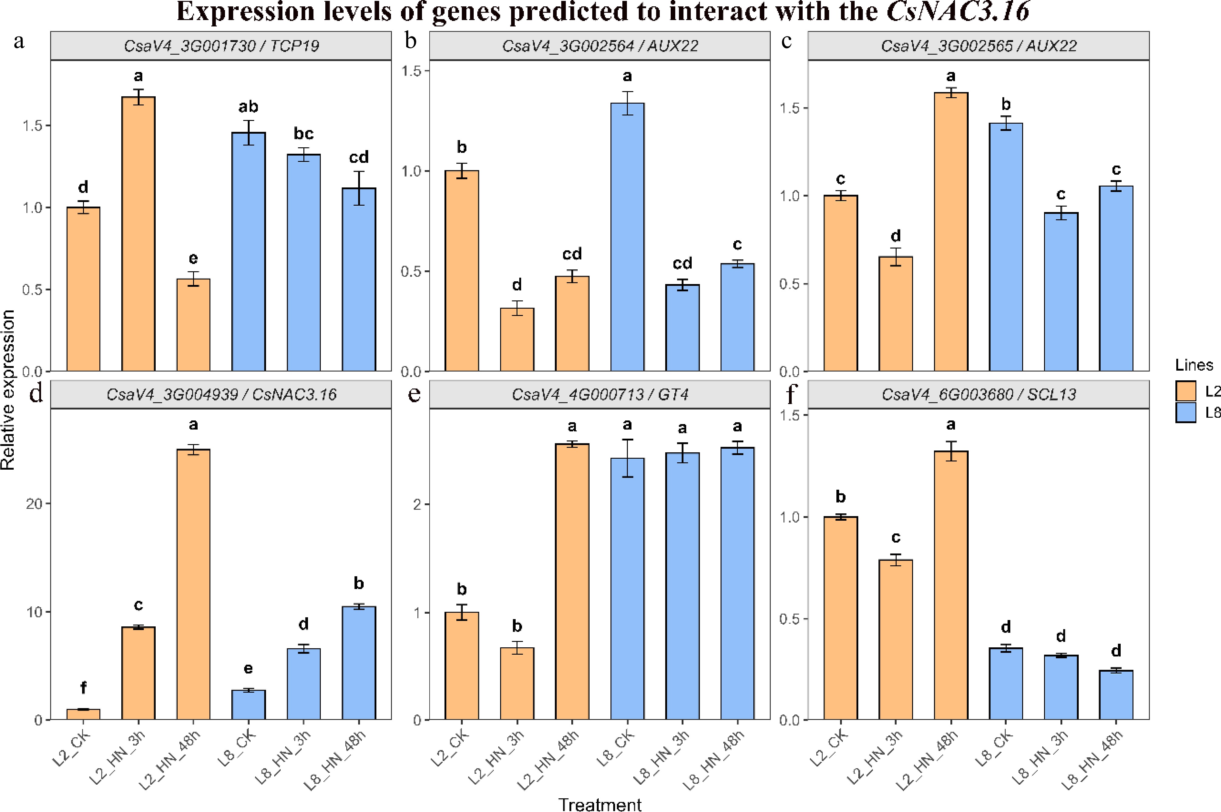
Figure 10.
Expression patterns of CsNAC3.16 and its predicted interacting genes under high nitrogen treatment. Relative expression levels were determined by qRT–PCR in the high-NUE line L2 and low-NUE line L8 under control conditions and after 3 and 48 h of high-nitrogen treatment. (a) CsaV4_3G001730; (b) CsaV4_3G002564; (c) CsaV4_3G002565; (d) CsNAC3.16 (CsaV4_3G004939); (e) CsaV4_4G000713; and (f) CsaV4_6G003680. Data are presented as mean ± SD (n = 3). Different lowercase letters indicate significant differences among treatments within the same genotype according to one-way ANOVA followed by Duncan's multiple range test (p < 0.05).
-
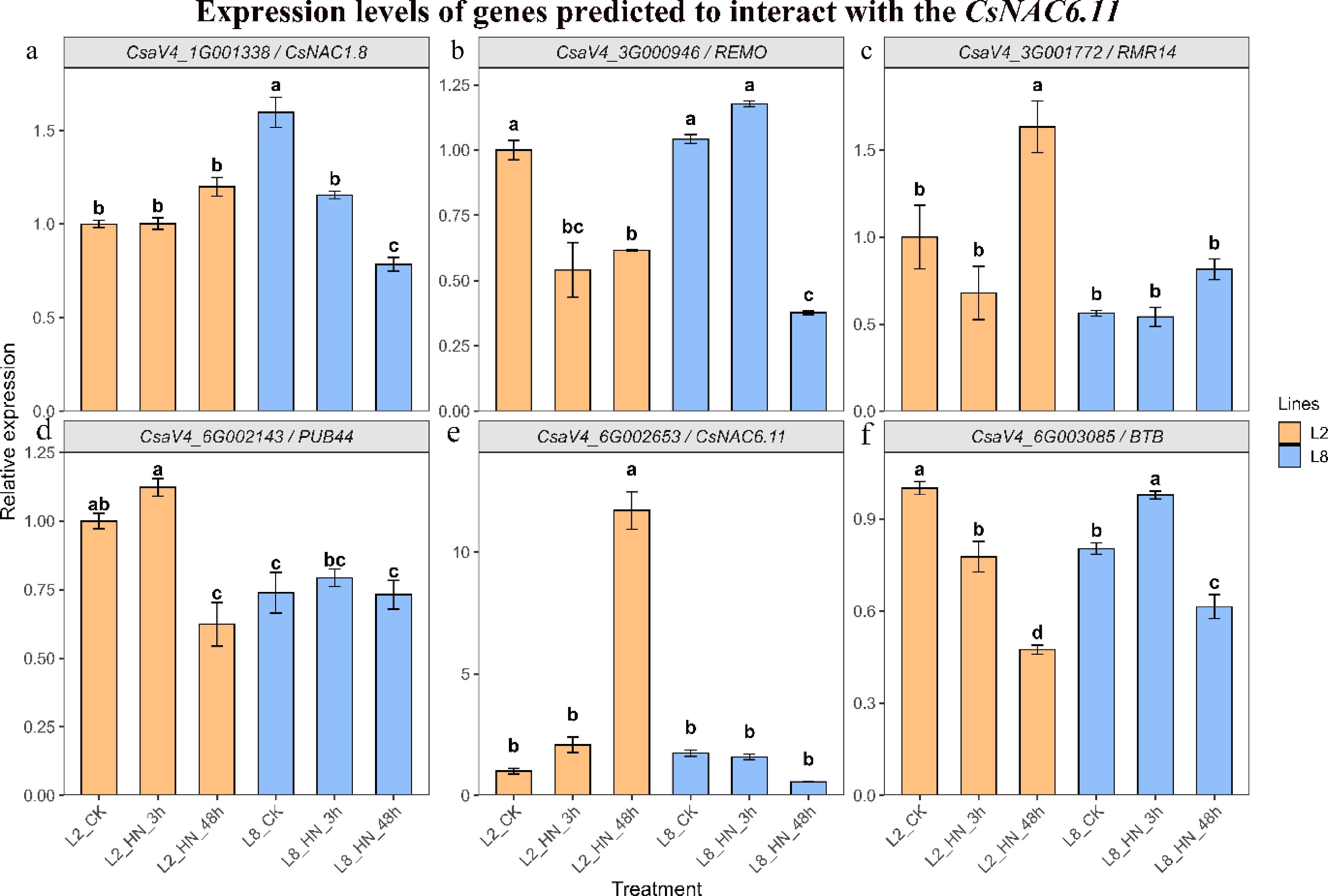
Figure 11.
Expression patterns of CsNAC6.11 and its predicted interacting genes under high-nitrogen treatment. Relative expression levels were determined by qRT–PCR in the high-NUE line L2 and low-NUE line L8 under control conditions and after 3 and 48 h of high-nitrogen treatment. (a) CsaV4_1G001338; (b) CsaV4_3G000946; (c) CsaV4_3G001772; (d) CsaV4_6G002143; (e) CsNAC6.11 (CsaV4_6G002653); and (f) CsaV4_6G003085. Data are presented as mean ± SD (n = 3). Different lowercase letters indicate significant differences among treatments within the same genotype according to one-way ANOVA followed by Duncan's multiple range test (p < 0.05).
Figures
(11)
Tables
(0)