-
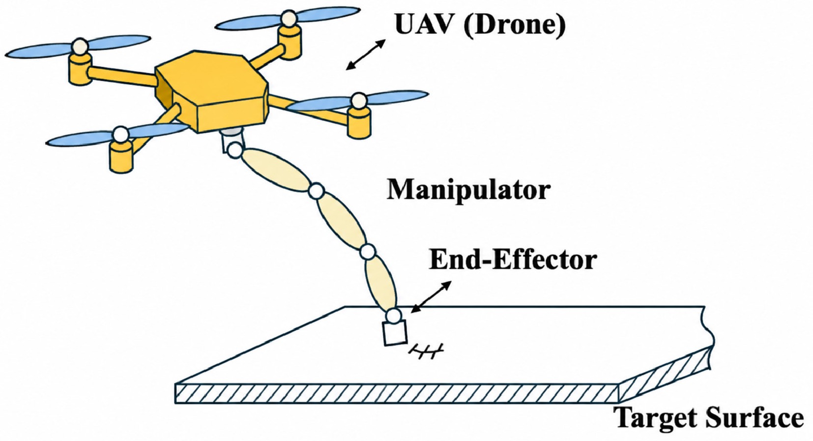
Figure 1.
Aerial manipulator performing contact-based surface interaction.
-
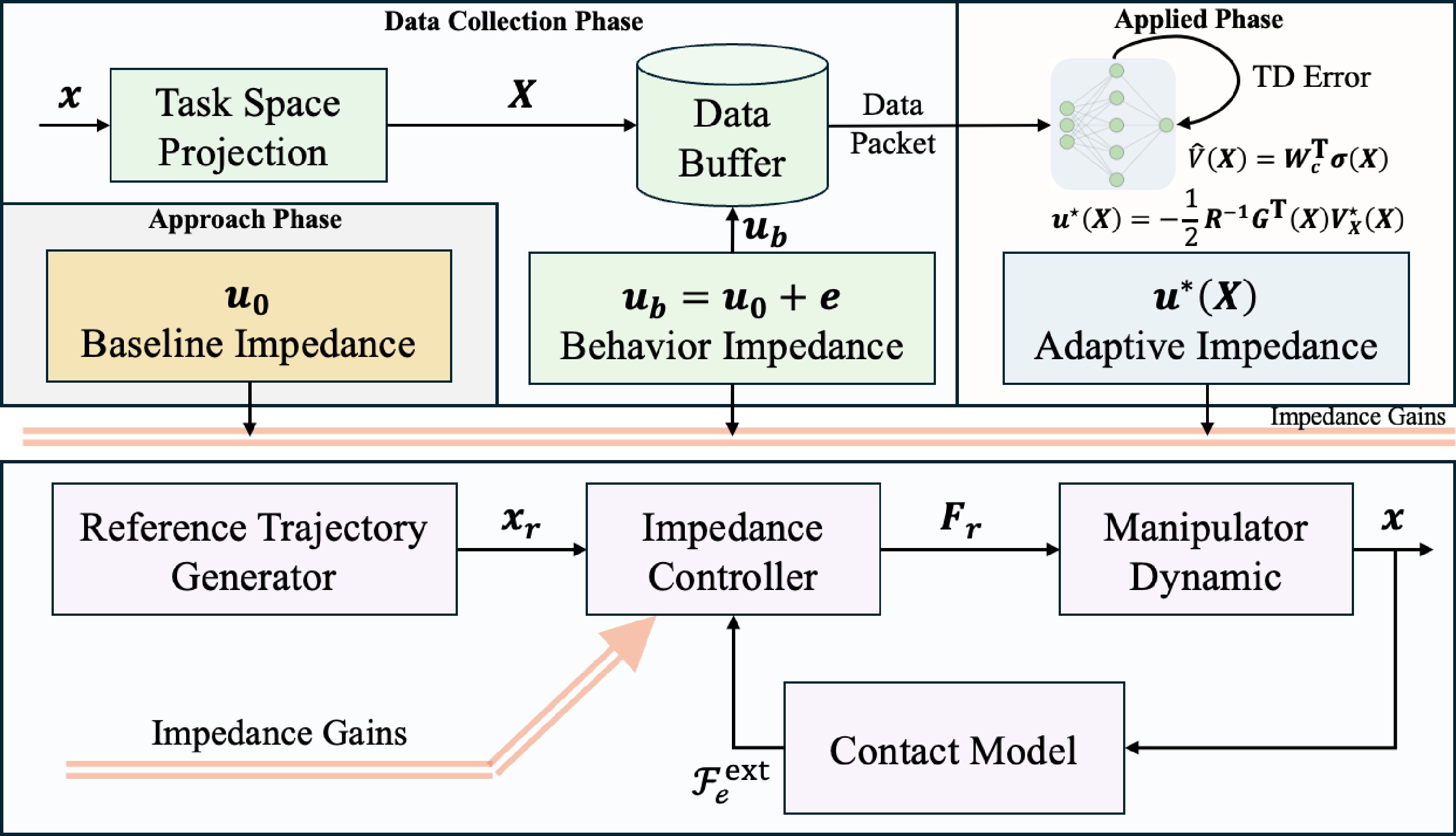
Figure 2.
Optimal adaptive impedance control framework.
-
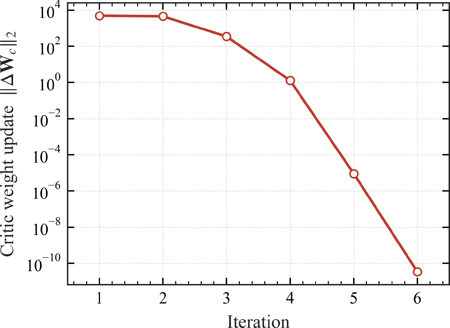
Figure 3.
Off-policy IRL convergence: per-iteration Critic-update norm
$ \|\Delta{\boldsymbol{W}}_{c}\|_{2} $ $ \varepsilon=10^{-6} $ -
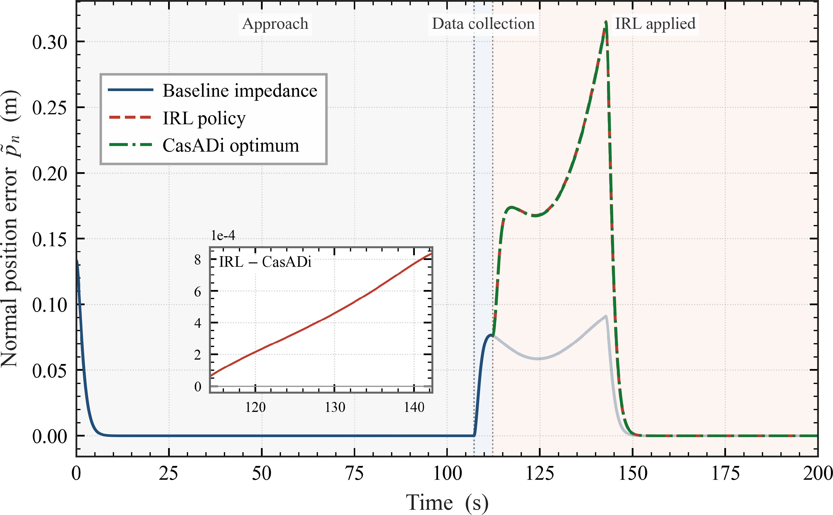
Figure 4.
Normal position error
$ \tilde p_{n}(t) $ $ - $ -
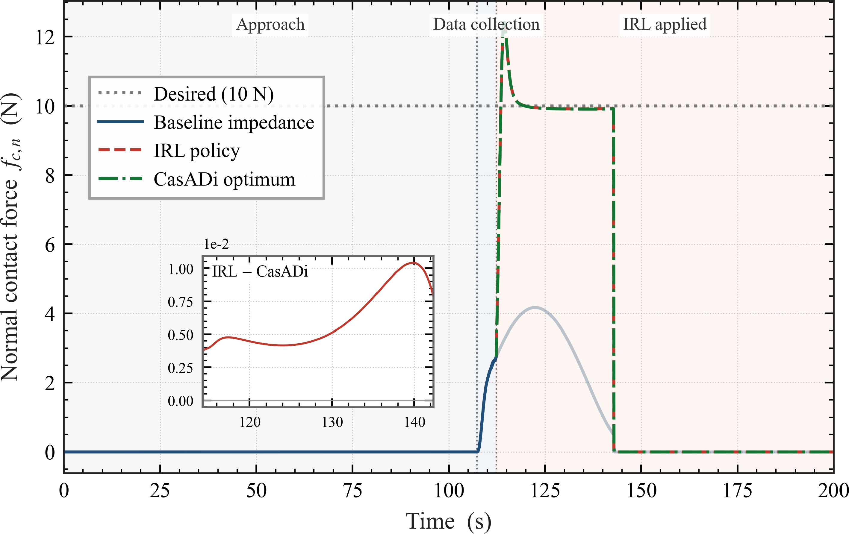
Figure 5.
Normal contact force
$ f_{c,n}(t) $ $ 10\,\mathrm{N} $ $ - $ -
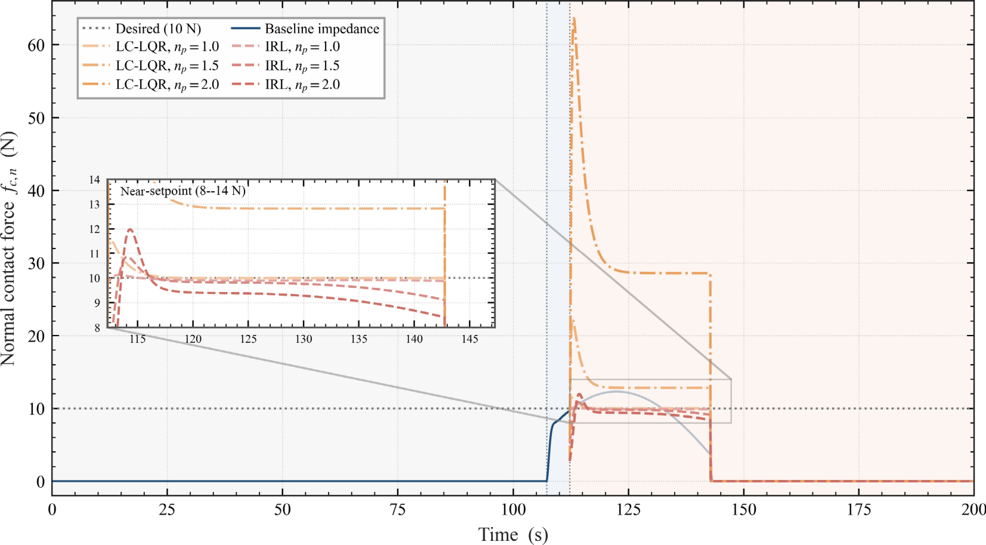
Figure 6.
Normal contact force
$ f_{c,n}(t) $ $ n_{p}\in\{1.0,1.5,2.0\} $ $ n_{p} $ $ \rightarrow $ $ n_{p} $ $ f_{d,n}=10\;\mathrm{N} $ $ 8 $ $ 14\;\mathrm{N} $ -
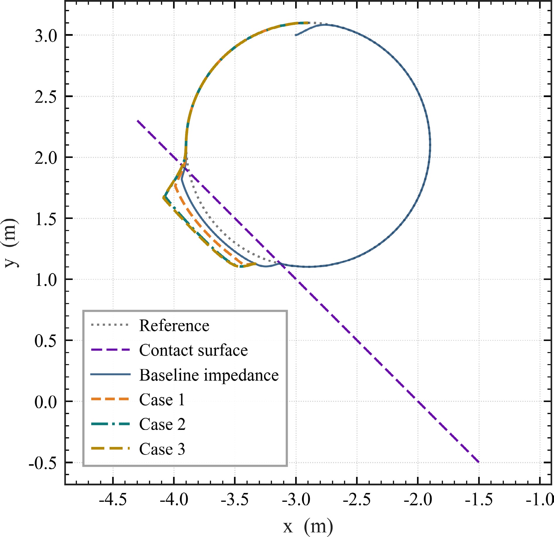
Figure 7.
End-effector path in the contact plane under the three weight configurations of Table 2, with the noisy baseline shown in light blue for reference.
-
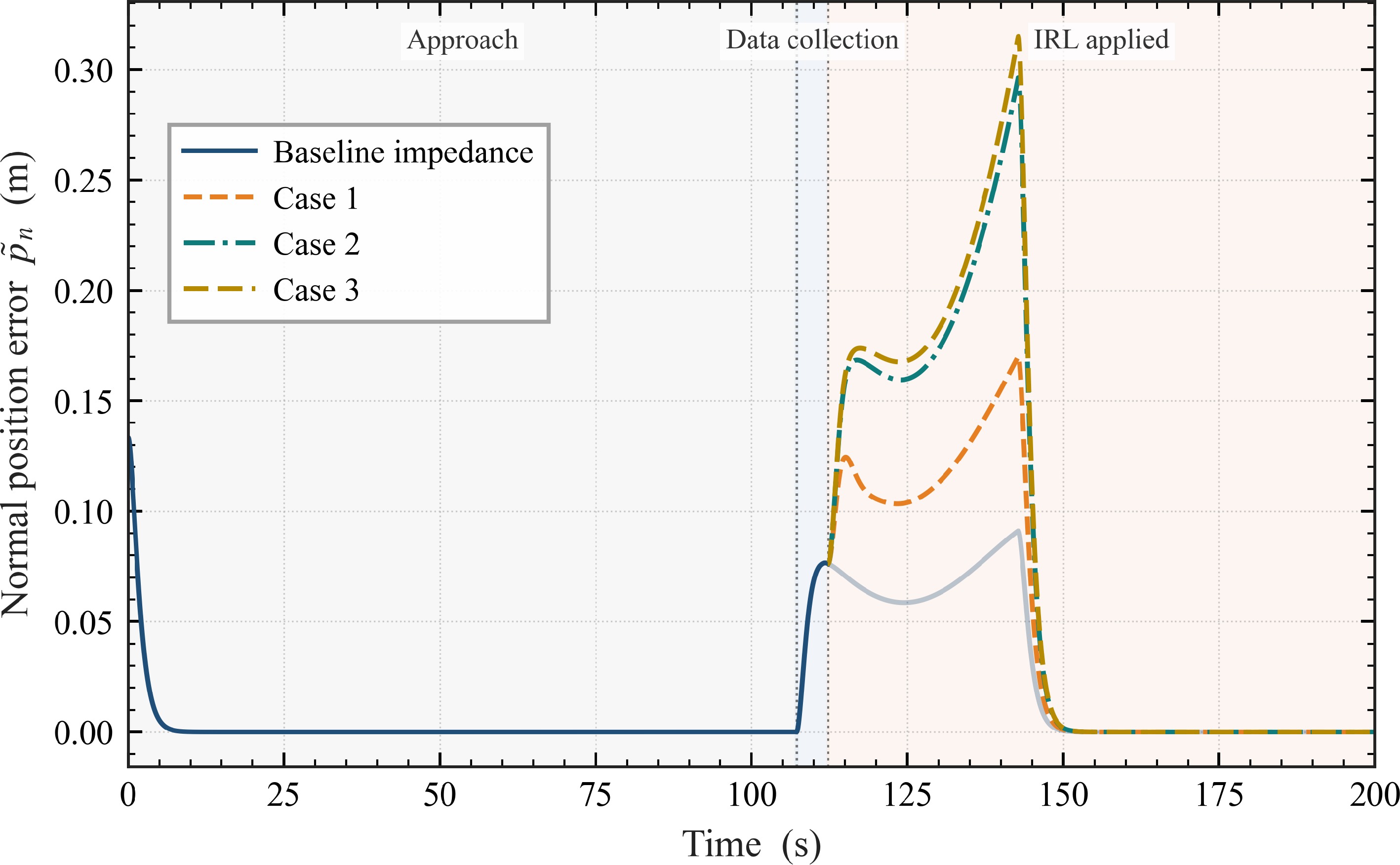
Figure 8.
Normal position error
$ \tilde p_{n}(t) $ -
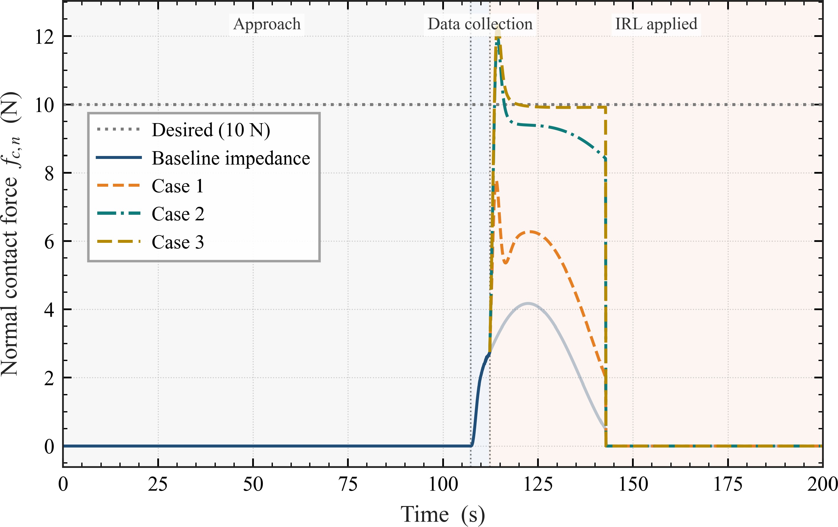
Figure 9.
Normal contact force
$ f_{c,n}(t) $ $ 10\,\mathrm{N} $ -
1: Choose discount factor $ \alpha $ $ {\boldsymbol{Q}},{\boldsymbol{R}} $ $ {\boldsymbol{\sigma}}({\boldsymbol{X}}) $ $ T_{\mathrm{int}} $ $ {\boldsymbol{W}}_{c}^{(0)} $ 2: Apply a stabilizing behavior policy $ {\boldsymbol{u}}_{b}={\boldsymbol{u}}_{0}+{\boldsymbol{e}} $ $ {\boldsymbol{u}}_{0} $ $ {\boldsymbol{e}} $ $ \{{\boldsymbol{X}}(t),{\boldsymbol{u}}_{b}(t)\} $ 3:for each trajectory segment $ [t_{k},t_{k}+T_{\mathrm{int}}] $ $ k=1,\dots,N $ 4: Form $ {\boldsymbol{\phi}}_{k} $ $ \Delta V_{k}^{(i)} $ 5: end for 6: Assemble $ {\boldsymbol{\Phi}}_{N} $ $ {\boldsymbol{\Delta}}_{N}^{(i)} $ 7: Update the Actor policy via (31). 8: Repeat steps 3–7 (re-forming the iteration-dependent targets along the same recorded trajectory) until $ \|{\boldsymbol{W}}_{c}^{(i+1)}-{\boldsymbol{W}}_{c}^{(i)}\|<\varepsilon $ 9: Deploy $ \hat{{\boldsymbol{u}}}^{\star}({\boldsymbol{X}}) $ $ \hat{{\boldsymbol{u}}}^{\star} $ $ \bigl(D_{n}^{\star}({\boldsymbol{X}}),K_{n}^{\star}({\boldsymbol{X}})\bigr) $ Table 1.
Off-policy IRL for optimal adaptive impedance control.
-
Parameter Value Description Simulation $ T $ $ 200\;\mathrm{s} $ Total simulation horizon $ \Delta t $ $ 0.01\;\mathrm{s} $ Sampling interval $ T_{\text{coll}} $ $ 5.01\;\mathrm{s} $ Exploration-noise window length End-effector initial condition $ {\boldsymbol{x}}_{0} $ $ [-3,\;3,\;0]^{\mathrm{T}}\;\mathrm{m} $ Initial end-effector position Reference trajectory generator (20) $ q $ $ 3 $ Auxiliary-state dimension $ {\boldsymbol{A}}_{d} $ $ \bigl[\begin{smallmatrix} 0 &\omega&0\\ -\omega&0&0\\ 0&0&0 \end{smallmatrix}\bigr],\;\omega=\pi/100\;\mathrm{rad/s} $ Exosystem dynamics matrix $ {\boldsymbol{C}}_{d} $ $ {\boldsymbol{I}}_{3} $ Exosystem output matrix $ {\boldsymbol{r}}_{d} $ $ [-0.066,\;-0.091,\;0]^{\mathrm{T}}\;\mathrm{m\;s^{-1}} $ Constant exosystem input $ {\boldsymbol{\zeta}}(0) $ $ [-2.9,\;3.1,\;0]^{\mathrm{T}}\;\mathrm{m} $ Initial auxiliary state Hunt–Crossley contact $ k_{c} $ $ 10^{2}\;\mathrm{N\;m^{-n_{p}}} $ Contact stiffness $ n_{p} $ $ 1.5 $ Deformation exponent, dimensionless (default) $ b_{c} $ $ 30\;\mathrm{s\;m^{-1}} $ Viscoelastic damping coefficient $ f_{d,n} $ $ 10\;\mathrm{N} $ Desired normal contact force $ {\boldsymbol{n}} $ $ [2,\;2,\;1]^{\mathrm{T}}/3 $ Outward surface normal (unit vector, tilted) $ {\boldsymbol{p}}_{e} $ $ [-3.5,\;1.5,\;0]^{\mathrm{T}}\;\mathrm{m} $ A point on the contact surface Baseline impedance (in the contact-attached frame) $ M_{n} $ $ 100\;\mathrm{kg} $ Baseline normal inertia $ D_{n}^{(0)} $ $ 200\;\mathrm{N\;s\;m^{-1}} $ Baseline normal damping $ K_{n}^{(0)} $ $ 100\;\mathrm{N\;m^{-1}} $ Baseline normal stiffness $ {\boldsymbol{M}}_{t} $ $ {\boldsymbol{I}}_{2}\;\mathrm{kg} $ Baseline tangential inertia $ {\boldsymbol{D}}_{t}^{(0)} $ $ 2{\boldsymbol{I}}_{2}\;\mathrm{N\;s\;m^{-1}} $ Baseline tangential damping $ {\boldsymbol{K}}_{t}^{(0)} $ $ {\boldsymbol{I}}_{2}\;\mathrm{N\;m^{-1}} $ Baseline tangential stiffness Off-policy IRL $ \alpha $ $ 0.01 $ Discount factor $ \deg({\boldsymbol{\sigma}}) $ $ 4 $ Polynomial critic basis order $ \sigma_{e} $ $ 0.1 $ Exploration-noise std (multiplicative on $ {\boldsymbol{u}} $ $ {\boldsymbol{Q}} $ $ \mathrm{diag}(5\times 10^{4},\;5\times 10^{4},\;0) $ State-cost weight (default) $ {\boldsymbol{R}} $ $ \mathrm{diag}(10^{-1},\;10^{-1}) $ Gain-cost weight (default) Table 1.
Simulation parameters used in the "Numerical simulation" section, grouped by category.
-
Case $ {\boldsymbol{Q}} $ $ {\boldsymbol{R}} $ $ 1 $ $ \mathrm{diag}(5\times 10^{4},\,5\times 10^{4},\,0) $ $ \mathrm{diag}(10^{-2},\,10^{-2}) $ $ 2 $ $ \mathrm{diag}(5\times 10^{4},\,5\times 10^{4},\,0) $ $ \mathrm{diag}(10^{-1},\,10^{-1}) $ $ 3 $ $ \mathrm{diag}(5\times 10^{-5},\,5\times 10^{-5},\,0) $ $ \mathrm{diag}(1,\,1) $ Cases are ordered by decreasing $ {\boldsymbol{Q}}/{\boldsymbol{R}} $ Table 2.
Cost-weight configurations for the sensitivity study.
Figures
(9)
Tables
(3)