Energy-efficient UAV−UGV coordinated control under line-of-sight maintenance constraint

Heterogeneous air-ground robotic teams often operate in a forward reconnaissance mode where a UAV advances ahead of a UGV, and cluttered environments can intermittently block visibility and communication, which motivates connectivity constraints that promote reliable coordination, including LOS^[1−3]. Such connectivity requirements can lead the UAV to perform energy-intensive maneuvers, including lateral detours, climbs, and frequent speed changes, which increase propulsion power demand and reduce endurance^[4], consistent with recent power consumption estimation results showing pronounced power variation under aggressive and time-varying kinematics^[5]. Recent MAV studies further emphasize the importance of real-time control, trajectory optimization, and onboard localization for small aerial platforms, including distributed nonlinear MPC for quadrotors, maneuverability-oriented trajectory optimization for fully actuated hexacopters, and moving-horizon UWB localization for small drones^[6−8]. As a result, UAV energy becomes a primary bottleneck for long-horizon operation, since the UAV battery capacity is typically far more limited than the UGV energy budget, and the UGV can often serve as a mobile depot for recharging and rendezvous scheduling to mitigate mission disruptions^[9,10]. The scenario is illustrated in Fig. 1. Motivated by this asymmetry, we treat the UGV trajectory as provided by a higher-level planner and focus on synthesizing UAV motion that satisfies LOS constraints while minimizing onboard energy, building on recent work in energy-efficient air-ground mission routing and minimum energy planning under periodic connectivity requirements^[11,12].

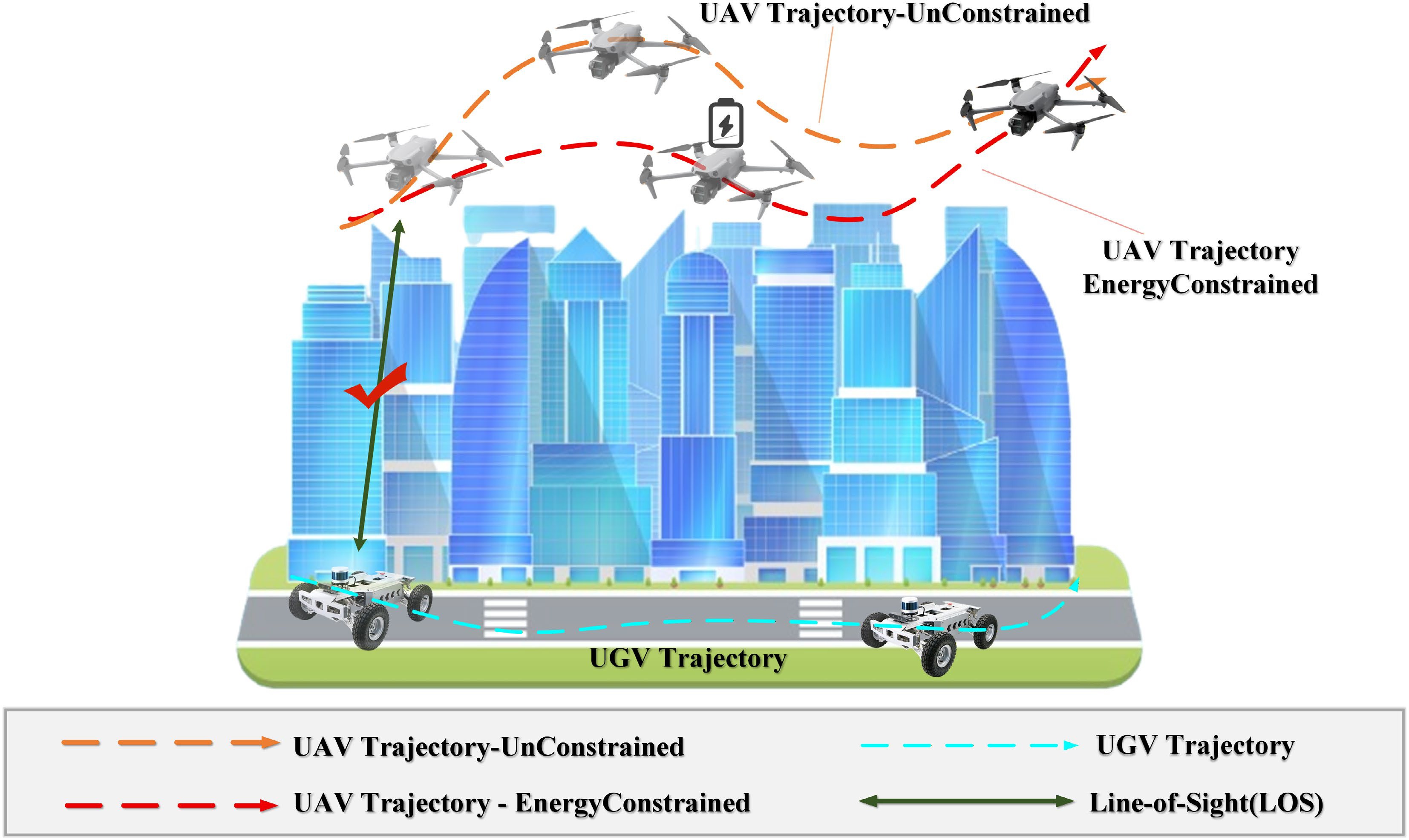
Figure 1. 

An illustration of a heterogeneous UAV and UGV systems operating in a cluttered environment. The UAV performs forward reconnaissance while maintaining LOS with the UGV and planning an energy-efficient trajectory toward the goal, accounting for LOS occlusions caused by obstacles.

A substantial literature studies coordination through formation and escort control and collaborative planning. Cheng et al. developed robust finite-time cooperative formation control under uncertainty and actuator faults^[13]. Klodt et al. imposed an explicit visibility constraint and showed that visibility requirements can reshape feasible relative motion^[14]. Papaioannou et al. incorporated explicit visibility constraints into UAV coverage planning by jointly optimizing guidance and sensing actions, providing a principled visibility-aware CPP formulation^[15]. Thelasingha et al. investigated iterative planning for energy-efficient cooperative task site assignments^[16]. Wen et al. mapped occlusion risk into online motion modulation to maintain LOS^[2]. For urban vehicular communication, ETAR further demonstrates that traffic-light-aware routing can exploit dynamic traffic information to improve routing efficiency and communication reliability^[17]. Adaptive reconfiguration via sampling-based reclustering for mMTC^[18] is complementary to the motion-level Shield presented in this paper. These studies provide effective coordination mechanisms, but they typically emphasize feasibility, and they do not directly minimize UAV motion energy under an explicit LOS-maintenance requirement when a UAV advances ahead of a UGV to conduct forward reconnaissance.

To clarify how LOS-maintenance requirements in forward reconnaissance can translate into energy-intensive detours and motion modulation, LOS maintenance can be viewed through visibility-aware motion planning, where occlusions are spatial, and the resulting visibility constraints can be non-smooth^[19,20]. Wang et al. developed visibility-aware trajectory optimization for aerial tracking by introducing optimization-friendly visibility costs, and further integrated visibility reasoning with additional constraints in cluttered scenes^[21,22]. Wang et al. also studied collaborative tracking in urban environments by explicitly accounting for occlusions to improve visibility during motion^[23]. Masnavi et al. proposed visibility-aware cooperative navigation that leverages visibility objectives in cluttered settings^[24], and Pritzl et al. studied cooperative navigation where a better-equipped platform guides an aerial vehicle through clutter while managing visibility constraints^[25]. These works provide practical mechanisms to represent occlusion and incorporate visibility into planning, but they primarily optimize visibility quality for perception and coordination rather than incorporating sampled LOS feasibility as an online motion-control requirement while minimizing UAV motion energy when a UAV advances ahead of a UGV to conduct forward reconnaissance. As a result, the energy impact of LOS-preserving detours, altitude changes, and speed modulation is often not co-optimized with the visibility objective, even though multirotor energy models, practical endurance-estimation methods, and flight-data-based energy-consumption prediction models are available^[26−28].

In parallel, multirotor energy modeling and energy-optimal planning have progressed from proxy objectives such as path length to system-level models and speed selection principles. Jacewicz et al. analyzed multirotor energy consumption using nonlinear dynamics and experimental evaluation^[29]. Bauersfeld & Scaramuzza derived analytic estimates for range, endurance, and optimal speed with experimental validation^[30]. Datsko et al. incorporated optimal speed selection into energy-efficient mission planning and reported substantial reductions in mission energy^[31]. Experimental studies on smaller platforms further relate flight conditions to power consumption^[32]. This energy bottleneck has also been recognized in larger networked UAV systems; for instance, intelligent UAV caching and energy management in 6G networks studies scalable energy-aware coordination for aerial communication services^[33]. However, most energy-focused results are developed without an explicit LOS-maintenance requirement for a moving ground partner, and they do not capture the energy penalties created by detours, climbs, and speed modulation that arise when LOS must be maintained in occlusion-rich environments.

Overall, prior work offers strong tools for cooperative control, visibility-aware planning, and multirotor energy modeling, but it does not provide a unified solution that directly minimizes UAV motion energy under constraint-consistent LOS maintenance in cluttered scenes. Existing approaches often enforce visibility or connectivity requirements without explicitly minimizing the UAV propulsion energy required to satisfy them, or they optimize energy without representing LOS constraints induced by complex occlusions. This paper addresses this gap by focusing on energy-minimizing UAV motion under LOS-aware feasibility enforcement when a UAV advances ahead of a UGV to conduct forward reconnaissance. The proposed Shield enforces sampled one-step feasibility when the admissible velocity set is non-empty and switches to a recovery action when the sampled constraints are temporarily infeasible.

To address the limited mission endurance caused by high propulsion energy demand in forward-reconnaissance UAV–UGV teams, this paper develops an energy-efficient and constraint-consistent control framework for cluttered environments. The framework reduces UAV propulsion energy while maintaining LOS connectivity. A learning-based controller outputs nominal velocity commands that are corrected by a Shield safety filter into executed velocities that respect safety-critical requirements, and all state propagation, energy accounting, and performance evaluation are defined on the executed shielded velocity to ensure that energy reduction is achieved in the closed loop. This design ensures that reduced UAV energy consumption translates into longer effective mission time under practical feasibility enforcement in deployment. The main contributions are summarized as follows:

● an energy-efficient motion control framework that integrates SAC-based nominal velocity generation with a real-time Shield to reduce UAV energy consumption while maintaining LOS connectivity and feasibility in cluttered environments;

● a propulsion-energy-aware shielded learning formulation for rotary-wing UAVs, built on a standard rotary-wing propulsion-power surrogate, that evaluates energy from the executed velocity and incorporates acceleration-related motion variation through executed-velocity smoothing and acceleration-sensitive model comparison;

● a real-time LOS connectivity evaluation method that integrates obstacle inflation with LOS segment sampling and applies smooth minimum aggregation to yield a continuous, differentiable LOS clearance margin for characterizing geometric occlusion risk.

The remainder of this paper is organized as follows. The proposed methodology and its practical implementation are described first, followed by the experimental setup and main results. The findings are then discussed, and the paper concludes with several directions for future research.

As illustrated in Fig. 2, the proposed framework forms a closed loop among the Environment module, the Energy-Efficient Constraint-Consistent Shielded Reinforcement Learning module, and the Task module.

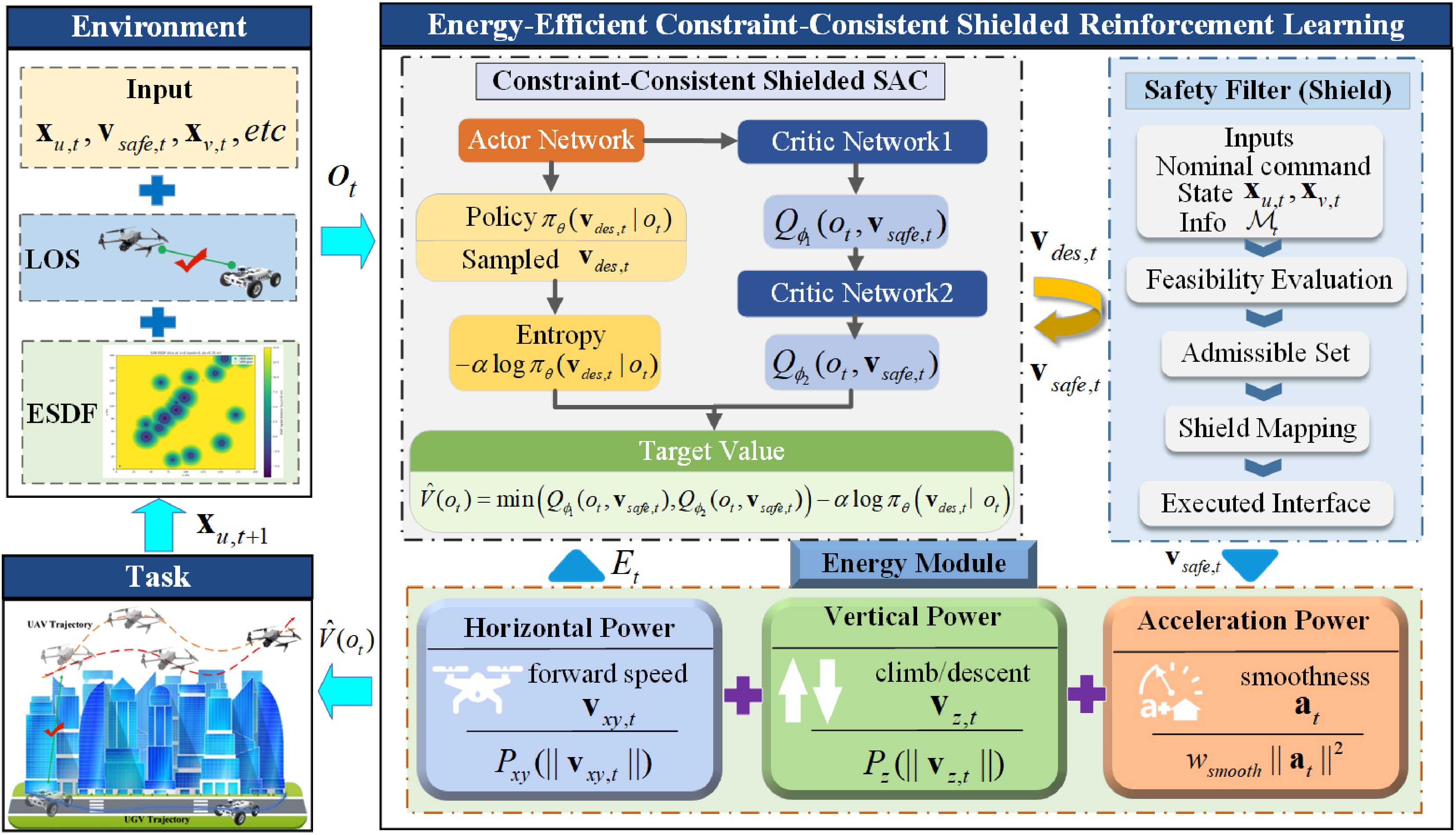
Figure 2. 

Framework of the proposed method.

At each time step, the Environment provides the current observation to the Learning module, which generates a nominal UAV velocity command. The Safety Filter, referred to as the shield, checks this command against safety and connectivity requirements and outputs the executed velocity. State propagation, energy accounting, reward evaluation, and termination checks are all computed from this shielded velocity rather than from the nominal command. Finally, the Task module updates the system and returns the next-state information to the Environment, completing the closed loop. This design keeps training and execution consistent under constraints and makes shield intervention explicitly measurable.

Problem formulation and kinematics

We consider a heterogeneous UAV–UGV team operating in a cluttered environment $ \Omega\subset\mathbb{R}^{3} $. The UGV is constrained to the ground plane, whereas the UAV can maneuver in 3D. The mission is forward reconnaissance: the UAV is required to stay ahead of the UGV in the horizontal projection, while maintaining LOS connectivity between the two platforms and avoiding collisions with obstacles. The primary objective is to reduce the UAV propulsion energy, subject to feasibility requirements imposed by collision avoidance, LOS maintenance, and motion limits.

In this work, the UGV trajectory is treated as an exogenous reference provided by a higher-level ground-vehicle or mission planner; thus, the proposed method focuses on the UAV-side motion-control problem. Joint UAV–UGV trajectory optimization, dynamic UGV replanning, and multi-agent task allocation are beyond the scope of the present study.

The control interface is velocity-based. At each time step, a policy generates a nominal velocity command, which is subsequently processed by a Safety Filter, denoted as the Shield, into an executed velocity. When the state-dependent admissible velocity set is non-empty, the Shield selects an executed command satisfying the one-step feasibility requirements. When no candidate velocity satisfies all requirements simultaneously, the Shield applies a recovery rule that prioritizes restoring LOS, obstacle-clearance, and forward-reconnaissance margins. Both state propagation and energy accounting are defined using the executed velocity, ensuring consistent evaluation when the nominal command is modified before execution. The Shield defines the actual control applied to the system and therefore the evaluation interface of the closed loop.

Time is discretized as $ t=0,1,\ldots,T-1 $ with sampling period $ \Delta t>0 $. The UAV and UGV positions are denoted by $ {\bf{x}}_{u,t},{\bf{x}}_{v,t}\in\mathbb{R}^3 $, respectively, with the ground constraint $ z_{v,t}\equiv 0 $ for the UGV. The feasible state spaces are:

$ {\cal{X}}_u $ and $ {\cal{X}}_v $ represent the admissible position sets for the UAV and UGV respectively.

Let:

denote the horizontal projection operator and the vertical unit vector, respectively.

Forward reconnaissance is formalized through an ahead requirement relative to the UGV in the horizontal projection. Using the horizontal projection operator $ P_{xy} $, define the UGV forward unit vector $ \hat{{\bf{t}}}_{v,t} $ using the direction to the UGV navigation goal $ {\bf{x}}_{v,g} $:

where, $ \|\cdot\|_2 $ is the Euclidean norm. The ahead distance is defined as the horizontal projection of the relative displacement onto the UGV forward direction:

$ s_{f,t} $ measures how far the UAV is ahead of the UGV along the UGV forward axis in the horizontal plane. The forward-reconnaissance requirement is imposed by:

where, $ s_{\min}>0 $ is a prescribed minimum ahead distance. A continuous violation magnitude is defined by the hinge form:

where, $ \sigma_{f,t}=0 $ indicates satisfaction of Eq. (5), and $ \sigma_{f,t}>0 $ quantifies the degree of violation.

Minimizing energy alone may lead to a trivial behavior where the UAV reduces motion to save power. To ensure a persistent task reference that advances with the UGV, we introduce a moving look-ahead reference point:

where, $ d_{{\rm{ahead}}}>0 $ is the desired look-ahead distance. The reference point $ {\bf{p}}_{{\rm{ref}},t} $ provides a time-varying target for defining progress-related terms in the learning formulation.

At each step t, the policy outputs a nominal UAV velocity command $ {\bf{v}}_{{\rm{des}},t}\in\mathbb{R}^{3} $. Since $ {\bf{v}}_{{\rm{des}},t} $ may violate feasibility conditions such as insufficient clearance to obstacles, degraded LOS margin, or violation of the forward-reconnaissance requirement, we introduce the Shield as the execution interface between the learning policy and the UAV dynamics. The Shield maps the nominal command to an executed velocity $ {\bf{v}}_{{\rm{safe}},t} $ according to:

where, $ {\cal{M}}_{t} $ summarizes the environment and task-related quantities used by the Shield, including obstacle-clearance information, LOS-margin information, the ahead-distance measure, the UGV reference velocity $ {\bf{v}}_{v,t} $, and motion-envelope parameters. The quantity $ {\cal{M}}_{t} $ is updated online at every control step using the latest available environmental and task information. Therefore, the Shield does not rely on a precomputed open-loop trajectory or a fixed obstacle configuration. When newly perceived obstacles, an updated ESDF, a changed LOS geometry, or a modified UGV reference velocity are available at time step t, they are incorporated into $ {\cal{M}}_{t} $ before the executable UAV command is selected.

The Shield is implemented as a one-step candidate-projection filter. Let:

denote the UAV velocity envelope. To construct candidate velocities, define a horizontal steering direction:

At each time step, a finite candidate set $ {\cal{C}}_t=\{{\bf{v}}_{t}^{k}\}_{k=1}^{K} $ is generated around the nominal command as:

Here, $ {\cal{A}} $, $ {\cal{B}} $, and $ {\cal{G}} $ are finite sets of speed-scaling factors, horizontal steering offsets, and vertical-velocity offsets, respectively. The operator $ \Pi_{{\cal{U}}}(\cdot) $ projects a candidate velocity onto the velocity envelope $ {\cal{U}} $, and the zero command provides a conservative braking or hovering candidate.

For each candidate $ {\bf{v}}\in{\cal{C}}_t $, the Shield predicts the one-step UAV and UGV states as:

The UGV prediction $ \hat{{\bf{x}}}_{v,t+1} $ is independent of the UAV candidate velocity because the UGV velocity $ {\bf{v}}_{v,t} $ is generated by the mission-level reference trajectory.

Using the predicted states, the Shield evaluates the predicted ahead distance, obstacle signed clearance, and LOS signed feasibility margin:

Here, $ \hat{s}_{f,t+1}({\bf{v}}) $ is computed from Eq. (4) using $ \hat{{\bf{x}}}_{u,t+1}({\bf{v}}) $ and $ \hat{{\bf{x}}}_{v,t+1} $; $ \hat{d}_{{\rm{obs}},t+1}({\bf{v}}) $ is the signed obstacle clearance evaluated at $ \hat{{\bf{x}}}_{u,t+1}({\bf{v}}) $; and $ \hat{g}_{{\rm{LOS}},t+1}({\bf{v}}) $ is the signed LOS feasibility margin evaluated on the segment between $ \hat{{\bf{x}}}_{u,t+1}({\bf{v}}) $ and $ \hat{{\bf{x}}}_{v,t+1} $.

The state-dependent admissible velocity set is then constructed as:

Here, $ z_{\min} $ and $ z_{\max} $ are the UAV altitude bounds, $ m_{{\rm{col}}} $ is the required collision-clearance margin, $ \varepsilon_{{\rm{LOS}}} $ is the required signed LOS margin, and $ s_{\min} $ is the minimum ahead distance. Because both the candidate set $ {\cal{C}}_t $ and the admissible set $ {\cal{V}}_t $ are reconstructed at each time step, the feasibility evaluation is reactive to the current observation rather than fixed by the initial map. Specifically, the predicted obstacle clearance $ \hat d_{{\rm{obs}},t+1}({\bf{v}}) $, the signed LOS margin $ \hat g_{{\rm{LOS}},t+1}({\bf{v}}) $, and the ahead-distance constraint $ \hat s_{f,t+1}({\bf{v}}) $ are re-evaluated for all candidate velocities using the latest states and environment information. Thus, if a newly detected obstacle or a change in UGV motion is reflected in the current observation, unsafe or LOS-violating velocity candidates can be removed from $ {\cal{V}}_t $ at the next control step.

When $ {\cal{V}}_{t}\neq\varnothing $, the executed command is selected as the admissible candidate that remains close to the nominal command while accounting for one-step energy and command smoothness:

Here, $ \widehat{E}_{t}({\bf{v}}) $ is the one-step propulsion-energy estimate obtained by substituting the candidate velocity $ {\bf{v}} $ into the UAV energy model, and $ \lambda_E,\lambda_{\Delta v}\ge 0 $ are weighting coefficients. For $ t=0 $, $ {\bf{v}}_{{\rm{safe}},t-1} $ is initialized as $ \mathbf{0} $.

When $ {\cal{V}}_{t}=\varnothing $, no candidate velocity in $ {\cal{C}}_t $ satisfies all one-step feasibility requirements simultaneously. In this case, the Shield applies a recovery command selected from the same candidate set:

Here, $ \eta_{{\rm{LOS}}},\eta_{{\rm{obs}}},\eta_f,\eta_v,\eta_{\Delta v}\ge 0 $ determine the relative priority of LOS-margin recovery, obstacle-clearance recovery, forward-reconnaissance recovery, conservative speed, and command smoothness.

Therefore, when $ {\cal{V}}_t \neq \varnothing $, the Shield enforces the stated sampled constraints for the selected candidate over the one-step prediction horizon. This property is conditioned on the current finite candidate set, the sampled LOS representation, and the latest available environment estimate. It should therefore be interpreted as sampled one-step feasibility rather than as an unconditional recursive-feasibility or hard LOS guarantee. When $ {\cal{V}}_t = \varnothing $, the executed command is determined by the recovery rule in Eq. (16), which prioritizes restoration of the feasibility margins.

With velocity-level kinematics, the system state is propagated by forward Euler integration:

where, $ {\bf{v}}_{{\rm{safe}},t} $ is the executed UAV velocity produced by the Shield in Eqs (8)–(16), $ {\bf{v}}_{v,t} $ is the UGV velocity generated by the mission-level reference trajectory, and $ \Delta t $ is the sampling period. The same executed velocity $ {\bf{v}}_{{\rm{safe}},t} $ is used later to compute step-wise energy and reward signals, avoiding ambiguity that would arise if nominal and executed commands were mixed. Concretely, all quantities that interact with the environment—including state transitions, energy accumulation, reward evaluation, and termination checks—are defined on $ {\bf{v}}_{{\rm{safe}},t} $ rather than on $ {\bf{v}}_{{\rm{des}},t} $.

Finally, to make the effect of feasibility enforcement explicit and to prevent attributing performance gains to the Shield itself, we quantify Shield intervention by:

which will be used both as a diagnostic metric and as a regularizer in the learning objective to discourage policies that rely on frequent post-corrections.

LOS geometry and risk metrics

Let $ \Omega\subset\mathbb{R}^3 $ denote the workspace and $ {\cal{O}}=\{{\cal{O}}_i\}_{i=1}^{N} $ the set of obstacles. Each obstacle $ {\cal{O}}_i $ is modeled as a vertical cylinder parameterized by its base center $ {\bf{o}}_i=[x_i,y_i,z_i]^{\top} $, radius $ R_i>0 $, and height $ H_i>0 $, with axial interval $ [z_i,\;z_i+H_i] $. Permitting $ z_i>0 $ captures elevated occluders, such as overhangs, that can block the LOS without occupying the ground plane.

The finite-cylinder obstacle model is adopted as a tractable abstraction of dominant LOS occluders in the considered simulation environment. This abstraction allows us to isolate and evaluate the coupling among UAV propulsion energy, LOS obstruction, altitude adjustment, and obstacle avoidance. However, it does not fully represent all urban occlusion geometries, such as irregular building facades, balconies, overhangs, vegetation, or detailed mesh structures.

To improve robustness to localization and mapping uncertainty, we introduce a nonnegative inflation margin $ b\ge 0 $ and uniformly inflate the radius:

where, $ \tilde{R}_i $ is the effective radius, and $ b=0 $ recovers the nominal geometry.

We define the clearance of a query point as its shortest Euclidean distance to the obstacle boundary. The corresponding signed distance is positive in free space and negative inside the inflated occupied set. Let $ \tilde{{\cal{O}}}=\bigcup_{i=1}^{N}\tilde{{\cal{O}}}_i $ denote the inflated occupied region with boundary $ \partial\tilde{{\cal{O}}} $. The Euclidean Signed Distance Field (ESDF) for any $ {\bf{p}}\in\Omega $ is defined as:

where, $ \|\cdot\|_2 $ is the Euclidean norm. Consequently, $ d_{{\rm{ESDF}}}({\bf{p}})>0 $ equals the clearance to the nearest obstacle boundary in free space, whereas $ d_{{\rm{ESDF}}}({\bf{p}})<0 $ indicates penetration and $ |d_{{\rm{ESDF}}}({\bf{p}})| $ is the penetration depth.

The UAV obstacle signed clearance at time t is defined as:

Correspondingly, the predicted obstacle signed clearance used by the Shield is $ \hat{d}_{{\rm{obs}},t+1}({\bf{v}}) = d_{{\rm{ESDF}}}(\hat{{\bf{x}}}_{u,t+1}({\bf{v}})) $.

For LOS assessment at discrete time t, given the UAV and UGV positions $ {\bf{x}}_{u,t} $ and $ {\bf{x}}_{v,t} $, we define the LOS segment as:

To obtain a computable approximation of the segment-to-obstacle relation, we uniformly sample $ S\ge 2 $ points on $ {\cal{L}}_{t} $:

where, $ {\bf{p}}(s_\ell)=[p_x,p_y,p_z]^{\top} $ is the $ \ell $-th sampled point.

For each sampled point $ {\bf{p}}(s_\ell)=[p_x,p_y,p_z]^{\top} $ and each inflated cylinder i, we compute the radial margin relative to the inflated radius $ \tilde{R}_i $:

and the vertical separation to the axial interval:

The radial margin $ \Delta_{i,r}(s_\ell) $ becomes negative when the sampled LOS point lies inside the inflated cylindrical radius. Therefore, using a sum-of-squares expression directly on $ \Delta_{i,r}(s_\ell) $ removes the penetration sign and may convert an occluded LOS sample into a positive clearance value. To avoid this ambiguity, we separate the LOS metric into two quantities: an unsigned proximity surrogate used for smooth risk shaping, and a signed feasibility margin used for LOS constraint checking.

The unsigned point-wise proximity surrogate is defined as:

The quantity $ \Delta_i^{+}(s_\ell) $ is nonnegative and is used only as a proximity/risk surrogate. In particular, when the sampled point lies inside the inflated cylinder and within its vertical interval, $ \Delta_i^{+}(s_\ell)=0 $, rather than producing a false positive clearance.

For feasibility checking, we further introduce a sign-preserving signed distance to the inflated finite cylinder. Let:

Define:

The signed distance to the inflated finite cylinder is then computed as:

where, the maximum between vectors is taken component-wise. This signed distance is positive outside the inflated cylinder, zero on its boundary, and negative inside it. Hence, it preserves the penetration sign required for LOS feasibility assessment.

To avoid the non-smoothness of a hard minimum, we approximate the minimum operator using a soft-min operator. For a vector $ {\bf{v}}=[v_1,\ldots,v_M] $, define:

which approaches $ \min_m v_m $ as $ \tau\to 0^{+} $.

Applying Eq. (30) to the unsigned proximity values gives the obstacle-wise minimum proximity surrogate:

The global unsigned LOS proximity surrogate is then defined as:

The quantity $ d_{{\rm{LOS}},t} $ is retained as a nonnegative proximity/risk indicator. A smaller $ d_{{\rm{LOS}},t} $ indicates that the LOS segment is closer to at least one occluder. However, it is not used as the signed feasibility margin.

In parallel, applying the soft-min aggregation to the signed cylinder distance yields the signed LOS feasibility margin:

The condition $ g_{{\rm{LOS}},t}>0 $ indicates that all sampled LOS points remain outside the inflated occupied cylinders, whereas $ g_{{\rm{LOS}},t}\le 0 $ indicates that at least one sampled LOS point lies on or inside an inflated obstacle. Therefore, $ g_{{\rm{LOS}},t} $ is used for LOS feasibility checking in the Shield and in the LOS violation term.

Finally, we map the unsigned LOS proximity surrogate $ d_{{\rm{LOS}},t} $, together with the signed feasibility margin $ g_{{\rm{LOS}},t} $, to a normalized LOS risk $ \phi_{{\rm{LOS}},t}\in[0,1] $. Given thresholds $ d_{{\rm{safe}}}>d_{{\rm{crit}}}\ge 0 $ and a shaping exponent $ p\ge 1 $, we define:

where:

and $ \bar{\xi}_t $ is obtained via a monotone $ C^1 $ cubic smoothstep:

The quantity $ d_{{\rm{LOS}},t} $ characterizes how close the LOS segment is to the obstacle when the sampled LOS remains safely outside the inflated occupied region. In contrast, $ g_{{\rm{LOS}},t}\le 0 $ directly indicates sampled LOS penetration or boundary contact and therefore saturates the LOS risk at one.

Energy-efficient constraint-consistent learning

Onboard battery capacity is limited, making UAV propulsion energy a key determinant of mission endurance. In contrast, the UGV typically has larger energy reserves, and its energy usage is not the dominant bottleneck in our setting. We therefore model energy consumption only for the UAV and use it as a physically grounded metric for both learning and evaluation.

The formulation is constraint-consistent: the policy is optimized with respect to the feasibility-adjusted action that is actually executed, and the objective explicitly regularizes the discrepancy between the proposed action and the feasible action. This reduces the mismatch between the optimization objective during learning and the behavior induced at deployment under safety and connectivity constraints.

For energy accounting, the UAV velocity at time step t is the executed velocity $ {\bf{v}}_{t}\equiv{\bf{v}}_{{\rm{safe}},t} $. We define the horizontal velocity component and the signed vertical velocity component using the same horizontal projection operator $ P_{xy} $ as in Eq. (2):

To avoid overloading $ P_{xy} $, which denotes the horizontal projection operator, we denote the horizontal propulsion power by $ P_{{\rm{hor}}}(\cdot) $. The horizontal propulsion power is given by a closed-form rotorcraft power model:

where, $ P_0 $ is the blade profile power in hover, $ P_i $ is the induced power in hover, $ U_{{\rm{tip}}} $ is the rotor tip speed, $ v_0 $ is the induced velocity in hover, $ d_0 $ is the fuselage drag ratio, ρ is air density, s is rotor solidity, and A is rotor disk area. The three terms capture profile losses, the nonlinear variation of induced power, and parasitic drag, respectively.

To account for three-dimensional maneuvers, we approximate the vertical power by a linear equivalent model:

where, $ k_{{\rm{climb}}} $ and $ k_{{\rm{desc}}} $ are equivalent power coefficients for climb and descent.

The total propulsion power and the step-wise energy are then:

where, $ \Delta t $ is the time step, $ E_t $ is the energy consumed at step t, and $ E_{{\rm{ep}}} $ is the cumulative episode energy. The $ \max(\cdot,0) $ enforces nonnegative consumption when energy regeneration is not considered.

The one-step energy estimate $ \widehat{E}_{t}({\bf{v}}) $ used by the Shield in Eq. (15) is computed by substituting a candidate velocity $ {\bf{v}} $ into Eqs (37)–(40). Thus, the same propulsion model is used consistently for both online Shield projection and reward evaluation.

Accordingly, $ E_t $, $ E_{{\rm{ep}}} $, and $ \widehat{E}_t({\bf{v}}) $ are model-based propulsion-energy estimates obtained from the executed velocity under the adopted horizontal and vertical power surrogates. They provide a consistent basis for comparing control policies under identical simulation settings, but they are not direct measurements of onboard battery discharge and should not be interpreted as guaranteed real-world battery savings without platform-specific power calibration.

We optimize a continuous-control policy by trading off task progress, soft feasibility violations, Shield intervention, and the UAV energy cost. The moving look-ahead reference point is defined in Eq. (7). The per-step progress signal is the reduction in distance from the UAV to this moving reference:

LOS connectivity is incorporated through the signed LOS feasibility margin $ g_{{\rm{LOS}},t} $ using a hinge-style violation:

Here, $ \varepsilon_{{\rm{LOS}}}>0 $ is the required signed LOS margin. Thus, $ \sigma_{{\rm{blk}},t}=0 $ means that the sampled LOS segment remains outside the inflated obstacles with at least $ \varepsilon_{{\rm{LOS}}} $ margin, while $ \sigma_{{\rm{blk}},t}>0 $ indicates insufficient signed clearance or sampled LOS penetration.

To discourage excessive post-correction and to bias the policy toward nominal commands that remain close to the admissible set, we use the Shield intervention magnitude $ I_t $ defined in Eq. (18) as a regularization term in the reward. The overall training and shielded execution procedure is summarized in Algorithm 1.

Putting everything together, the per-step return is:

where, the $ w_{\cdot} $ terms are scalar weights and $ \mathbb{I}\{\cdot\} $ is the indicator function. The smoothness term is computed from the executed velocity rather than the nominal velocity, which is consistent with the closed-loop state transition in Eq. (17). The reward weights also determine the trade-off between propulsion-energy reduction and mission completion time. The energy weight $ w_E $ penalizes step-wise propulsion energy and therefore encourages smoother and lower-power motion. In contrast, the progress weight $ w_{{\rm{prog}}} $, the time penalty $ w_{{\rm{time}}} $, and the goal-reaching reward $ w_{{\rm{goal}}} $ encourage the UAV to maintain task progress and complete the mission efficiently. As a result, the framework avoids minimizing energy alone. A policy that slows down excessively or hovers to save energy would accumulate the time penalty and receive less progress reward. By increasing $ w_E $, the framework can be configured toward endurance-prioritized operation, whereas increasing $ w_{{\rm{prog}}} $, $ w_{{\rm{goal}}} $, or the relative influence of $ w_{{\rm{time}}} $ shifts the behavior toward time-prioritized operation.

We learn a parametric policy $ \pi_\theta(\cdot \mid o_t) $ under observation $ o_t $ by maximizing the expected discounted return:

This formulation treats physically grounded UAV energy $ E_t $ as the primary cost while keeping progress, LOS connectivity, ahead behavior, collision avoidance, and Shield intervention aligned through explicitly defined violations and regularization terms.

The online computational cost of the Shield is determined by the number of candidate velocities $ K=|{\cal{C}}_t| $, the number of obstacles N, and the number of LOS samples S. For each candidate velocity, the Shield evaluates the one-step altitude, obstacle-clearance, ahead-distance, and LOS-margin constraints. Since LOS checking evaluates S sampled points against N obstacles, the per-step Shield complexity is $ O(KNS) $. The SAC actor inference cost is denoted by $ O(P_{\theta}) $, where $ P_{\theta} $ is the policy-network size. Therefore, the overall online control complexity is $ O(P_{\theta}+KNS) $. For a fixed candidate design and map representation, K, N, and S are bounded, making the online execution cost predictable.

To validate the proposed UAV–UGV coordination framework under the LOS maintenance constraint, we conduct four studies under constraint-consistent execution. First, we evaluate a constraint-inactive scenario to confirm that energy reduction mainly comes from the learned policy rather than Shield interventions. Second, we perform a propulsion-energy ablation to verify the benefit of including the executed-velocity energy cost in the learning objective. Third, we conduct a disturbance-aware dynamic validation to test whether the energy-saving trend remains under command delay, velocity-response lag, and wind disturbance. Fourth, we compare three propulsion-energy models under identical task settings and feasibility checking. We also profile the online runtime of the trained SAC–Shield controller to verify the computational tractability of the shielded execution interface.

Energy reduction under inactive constraints

We study a setting in which the collision-avoidance and LOS-connectivity constraints are satisfied with ample margins throughout the episode, yielding negligible Shield interventions. Vme serves as the baseline because it is the constant cruise speed that minimizes energy per unit distance under the same propulsion model.

Accordingly, collision and LOS constraints encoded by the admissible set in Eq. (14) remain inactive for most of the episode. The UAV and UGV evolve under the kinematics in Eq. (17), and the executed action is obtained via the Shield mapping in Eq. (8). Energy is evaluated on the executed velocity using Eq. (40). We compare three methods:

● FAST: time-prioritized tracking of $ {\bf{p}}_{{\rm{ref}},t} $ by flying at $ v_{\max} $, with altitude held constant.

● Vme: tracking $ {\bf{p}}_{{\rm{ref}},t} $ with a constant cruise speed $ V_{{\rm{me}}} $ that minimizes energy per unit distance under the same propulsion model.

● Ours: a learned policy whose desired command is filtered by the Shield, with energy computed from the executed command.

All methods share the same parameters: $ \Delta t=0.1\,{\rm{s}} $, $ v_{\max}=15\;\mathrm{m/s} $, $ z_0=10\;{\rm{m}} $, $ y_{{\rm{bound}}}=\pm 30\;{\rm{m}} $, $ L=200\,{\rm{m}} $, and horizon $ T=3,000 $. The UGV speed is $ v_g\in\{8,10\}\;\mathrm{m/s} $ 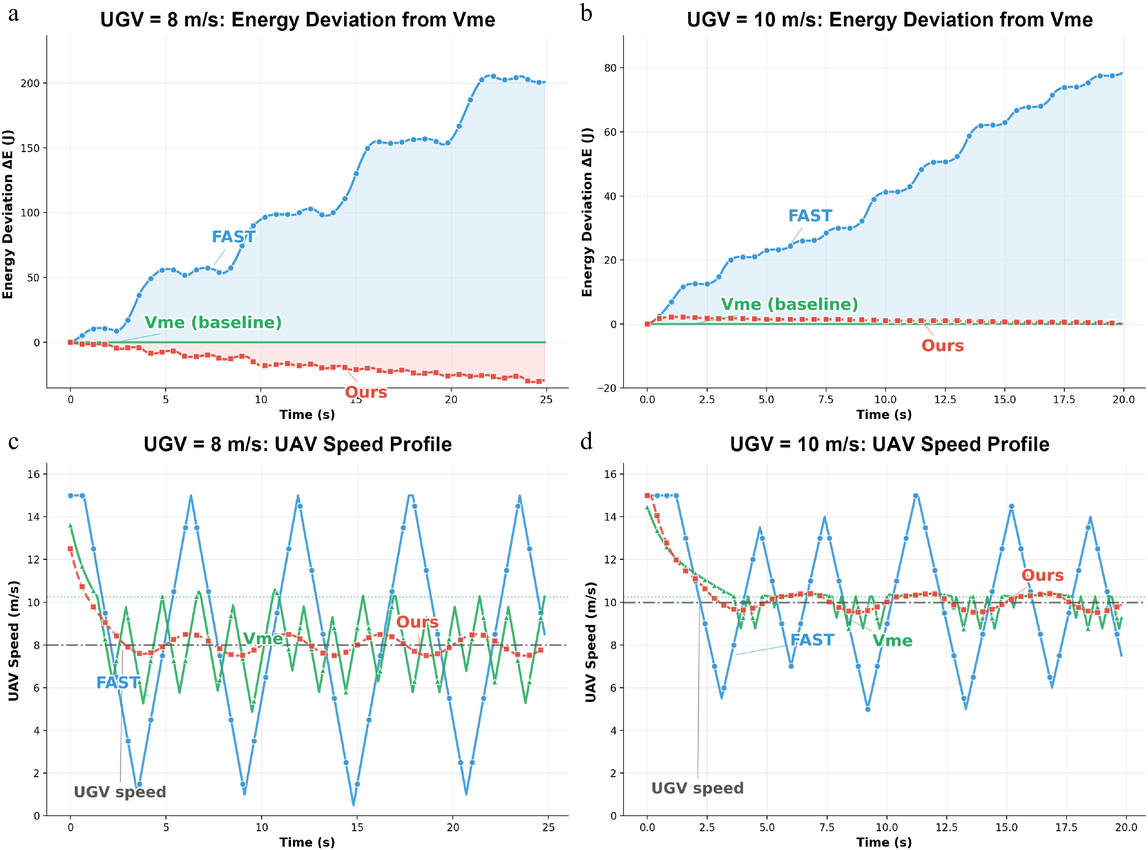with a small sinusoidal perturbation. The cumulative energy deviation and the corresponding UAV speed profiles are shown in Fig. 3.

Figure 3. 

Constraint-inactive comparison relative to Vme. (a), (b) Cumulative energy deviation $ \Delta E(t) $ from the Vme baseline for $ v_g\in\{8,10\}\,\mathrm{m/s} $ over the full episode. (c), (d) Corresponding UAV speed profiles under the same setting.

As shown in Fig. 3a and b, for $ v_g=8\;\mathrm{m/s} $, Ours achieves lower cumulative energy than Vme and markedly improves over FAST. The speed profiles in Fig. 3c and d show that Ours maintains a smooth speed concentrated near the task-relevant cruise band, while FAST exhibits frequent near-$ v_{\max} $ bursts. For $ v_g=10\;\mathrm{m/s} $, Ours remains close to the Vme baseline while still reducing energy relative to FAST. Shield interventions remain negligible in both runs.

These results illustrate the energy–time trade-off induced by different speed-selection strategies. FAST represents a time-prioritized strategy, whereas Vme represents an energy-per-distance cruise strategy. The proposed method avoids unnecessary high-speed oscillations while maintaining task progress, reflecting a tunable compromise between operational speed and energy efficiency.

Propulsion energy model ablation

This experiment ablates the propulsion-energy term in the learning objective and isolates its effect under the safety-filtered execution pipeline. At each time step, the policy outputs a nominal velocity command, which is then passed through the Shield to produce an executed velocity $ {\bf{v}}_{{\rm{safe}},t} $. We compare EnergyConstrained, which includes the energy cost by setting $ w_E>0 $, with Unconstrained, which removes this term by setting $ w_E=0 $. Both methods use the same Shield at execution time, and all reported energy is computed from the executed velocity. Experiment parameters are summarized in Table 1.

For evaluation, propulsion power is computed from $ {\bf{v}}_{{\rm{safe}},t} $ using the rotorcraft horizontal power model in Eq. (38) and the vertical power model in Eq. (39). We report the energy-saving ratio:

To reduce bias from different completion times, cumulative energy is aligned by UAV trajectory arc length:

Scenario 1 starts from an initial NLOS condition and requires LOS recovery while navigating the corridor. The planar trajectories are shown in Fig. 4. As shown in Fig. 4, both methods complete the traversal, while EnergyConstrained follows a feasible route with less aggressive local deviations. The corresponding altitude evolution and LOS clearance are presented in Fig. 5.

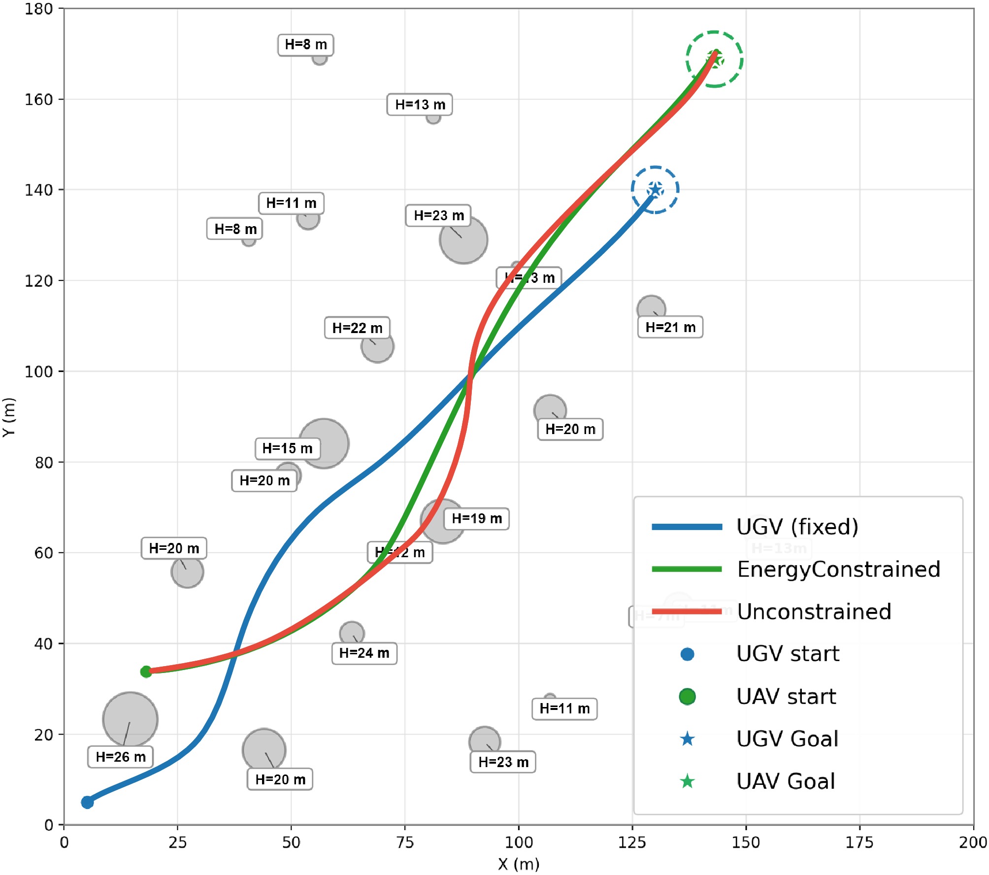
Figure 4. 

Scenario 1 (initial NLOS): planar trajectories of the UGV and UAV.

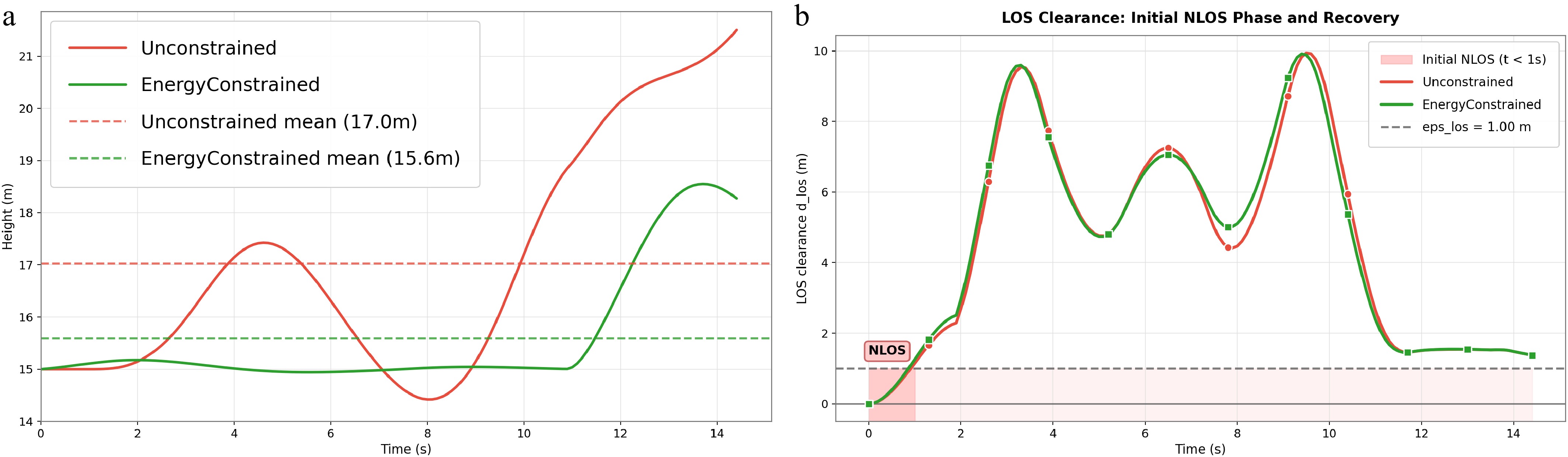
Figure 5. 

Scenario 1 (initial NLOS): altitude evolution and LOS clearance for Unconstrained and EnergyConstrained. (a) UAV height profiles. (b) LOS clearance/margin metric.

Figure 5 shows that EnergyConstrained maintains a lower mean altitude while recovering LOS clearance above $ \varepsilon_{\rm{LOS}}=1.0\rm{\ m} $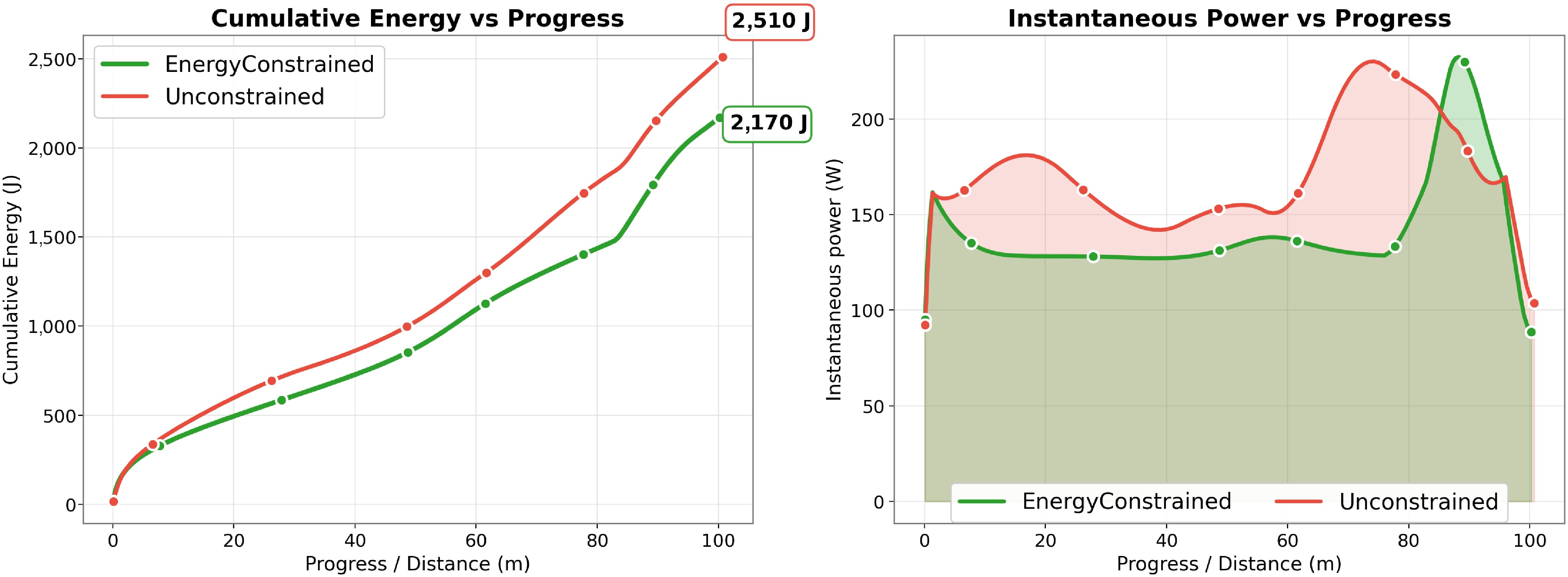, indicating that LOS restoration is achieved without excessive climbing or unnecessary vertical oscillations. The progress-aligned energy and instantaneous power are shown in Fig. 6, providing a direct comparison of cumulative consumption, transient power demand, and the energy advantage obtained along comparable mission progress.

Figure 6. 

Scenario 1 (initial NLOS): cumulative propulsion energy aligned by progress and instantaneous power computed from executed velocities using Eq. (40).

As shown in Fig. 6, at the same progress, EnergyConstrained reduces cumulative energy from $ 2,510\rm{\ J} $ to $ 2,170\ \rm{J} $, yielding $ \eta_E=13.5{\text{%}} $.

Scenario 2 starts from an initial LOS condition in a more cluttered environment. The planar trajectories are shown in Fig. 7.

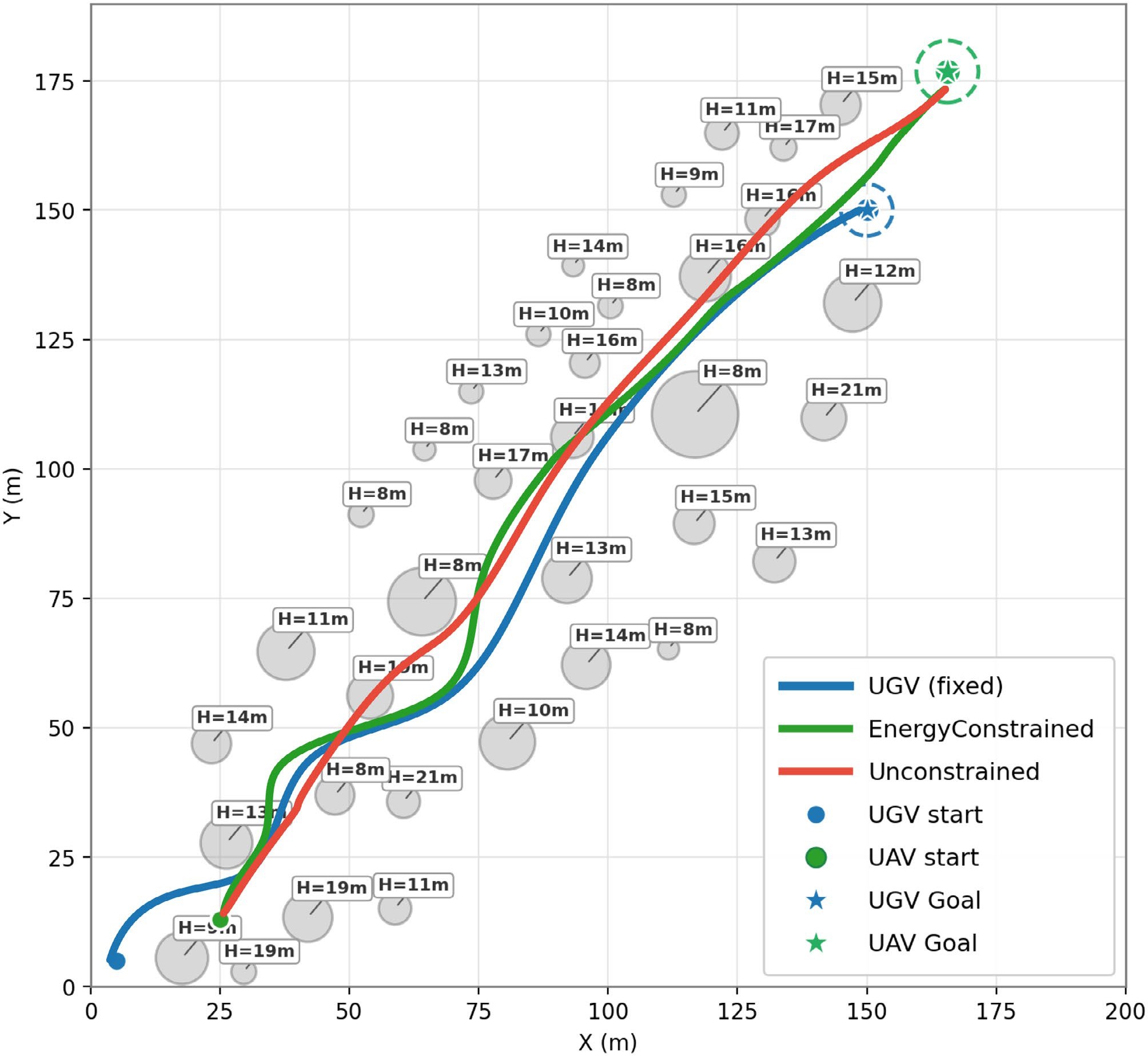
Figure 7. 

Scenario 2 (initial LOS): planar trajectories of the UGV and UAV in a cluttered urban environment with multiple obstacles.

Figure 7 shows that both methods reach the goal through similar corridors, while EnergyConstrained yields smoother local adjustments and avoids unnecessary lateral detours in the cluttered region. The altitude and LOS profiles are shown in Fig. 8, further illustrating the corresponding vertical-motion behavior and connectivity-maintenance performance.

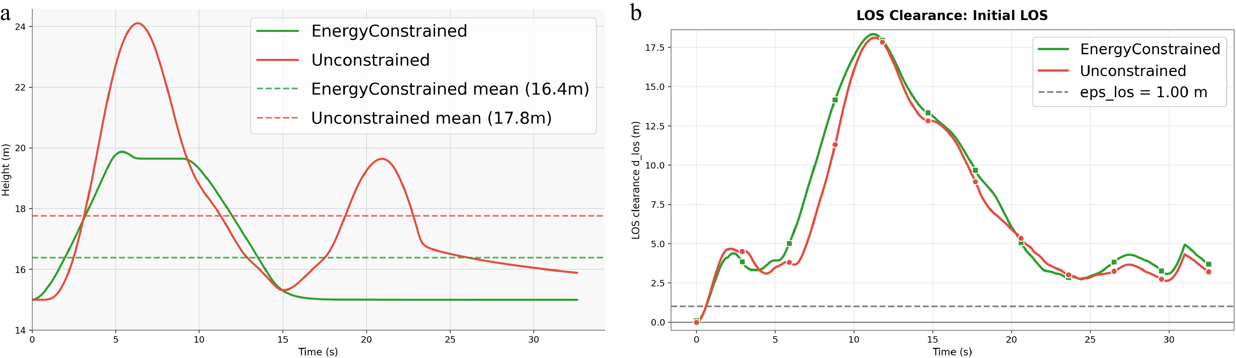
Figure 8. 

Scenario 2 (initial LOS): altitude evolution and LOS clearance for Unconstrained and EnergyConstrained. (a) UAV height profiles. (b) LOS clearance/margin metric.

Figure 8 further shows that EnergyConstrained maintains a lower mean altitude while keeping the LOS clearance above the required margin. The progress-aligned energy and instantaneous power are shown in Fig. 9.

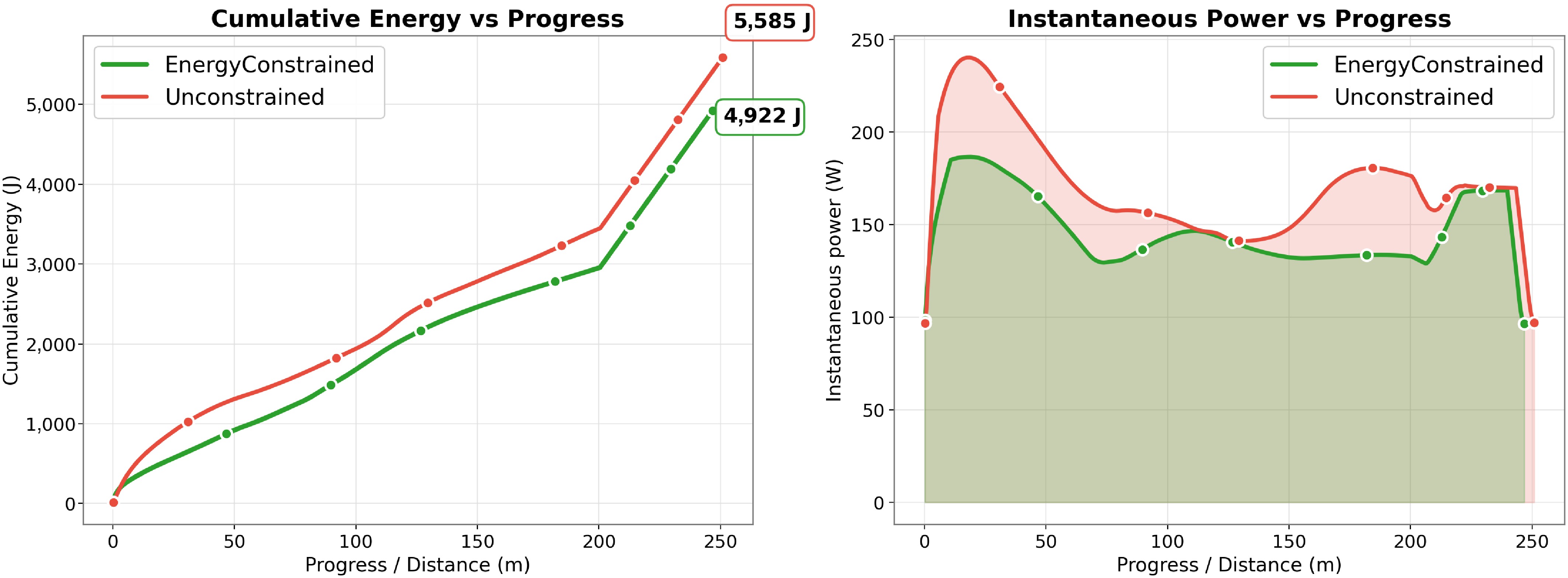
Figure 9. 

Scenario 2 (initial LOS): cumulative propulsion energy aligned by progress and instantaneous power computed from executed velocities using Eq. (40).

As shown in Fig. 9, EnergyConstrained reduces cumulative energy from $ 5,585\rm{\ J} $ to $ 4,922\ \rm{J} $, corresponding to $ \eta_E=11.9{\text{%}} $. The relative saving is smaller than in Scenario 1, which is consistent with reduced flexibility in a denser environment.

For an illustrative battery-budget interpretation, the propulsion-energy reduction can be mapped to a surrogate-based relative endurance proxy under the same usable-battery and reserve-energy assumptions. Let $ E_{bat}^{use} $ denote the assumed usable onboard battery energy and $ E_{res} $ the assumed reserve energy. For an operating mode with average propulsion power $ \bar{P} $, the corresponding idealized operation time can be estimated as:

For a progress-aligned mission segment, the relative endurance gain induced by an energy-saving ratio $ \eta_E $ is approximated by:

Under these idealized battery-budget assumptions, the energy reductions of 13.5% and 11.9% correspond to surrogate-based relative endurance proxies of approximately 15.6% and 13.5%, respectively. This calculation is not a prediction of real flight duration or battery discharge, which would require platform-specific battery, payload, and power-system measurements.

Disturbance-aware dynamic validation

To examine whether the energy-saving trend is sensitive to idealized kinematic execution, we further conduct a disturbance-aware dynamic validation. This experiment does not replace real flight tests or high-fidelity hardware-in-the-loop validation, but tests whether the proposed energy-aware shielded execution remains beneficial when command delay, velocity-response lag, and wind disturbance are introduced during evaluation.

At each time step, the Shield first produces the feasible command $ {\bf{v}}_{{\rm{safe}},t} $ using the same execution interface defined in Eq. (8). The delayed Shielded command is defined as:

where, d is the command delay measured in control steps. The delayed command is then passed through a first-order velocity-response model:

where, $ \tau_{{\rm{v}}} $ is the velocity-response time constant and

The initial actual velocity $ {\bf{v}}_{{\rm{act}},0} $ is initialized by the delayed command.

A horizontal wind disturbance $ {\bf{v}}_{{\rm{wind}},t} $ is added during UAV position propagation:

The UGV still follows the reference update in Eq. (17). For energy evaluation, propulsion power is recomputed from the wind-relative airspeed:

The disturbed step-wise propulsion energy is computed as

Three execution cases are considered. The Ideal case uses $ d=0 $, $ \tau_{{\rm{v}}}=\infty $, and zero wind. The Mild case uses $ d=1 $, $ \tau_{{\rm{v}}}=0.3\,{\rm{s}} $, and mean horizontal wind magnitude $ 2.8\,\mathrm{m/s} $. The Strong case uses $ d=2 $, $ \tau_{{\rm{v}}}=0.2\,{\rm{s}} $, and mean horizontal wind magnitude $ 5.7\,\mathrm{m/s} $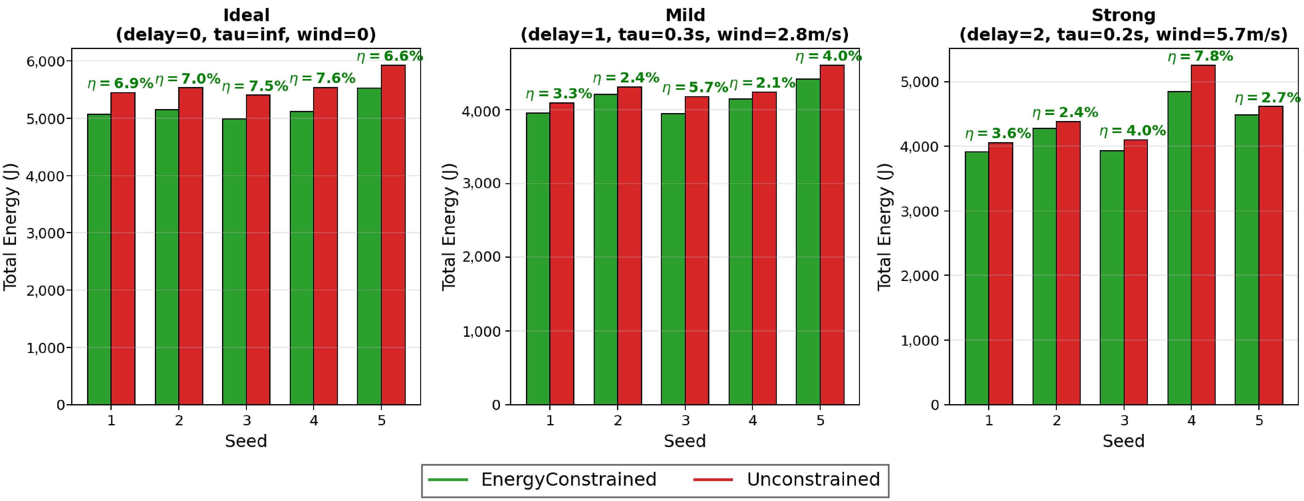. For each case, five random seeds are evaluated with the same obstacle generation, LOS threshold, Shield feasibility checking, and energy-evaluation interface. The resulting energy-saving comparison is reported in Fig. 10.

Figure 10. 

Energy comparison under ideal, mild-disturbance, and strong-disturbance execution. A positive $ \eta_E $ indicates that EnergyConstrained consumes less total propulsion energy than Unconstrained under the same disturbance case.

As shown in Fig. 10, EnergyConstrained consistently consumes less propulsion energy than Unconstrained in all three execution cases. The average energy-saving ratios are 7.13%, 3.51%, and 4.11% under Ideal, Mild, and Strong execution, respectively. Although the saving ratio decreases after introducing delay, velocity-response lag, and wind disturbance, the energy-saving trend remains positive. The corresponding LOS safety statistics are shown in Fig. 11.

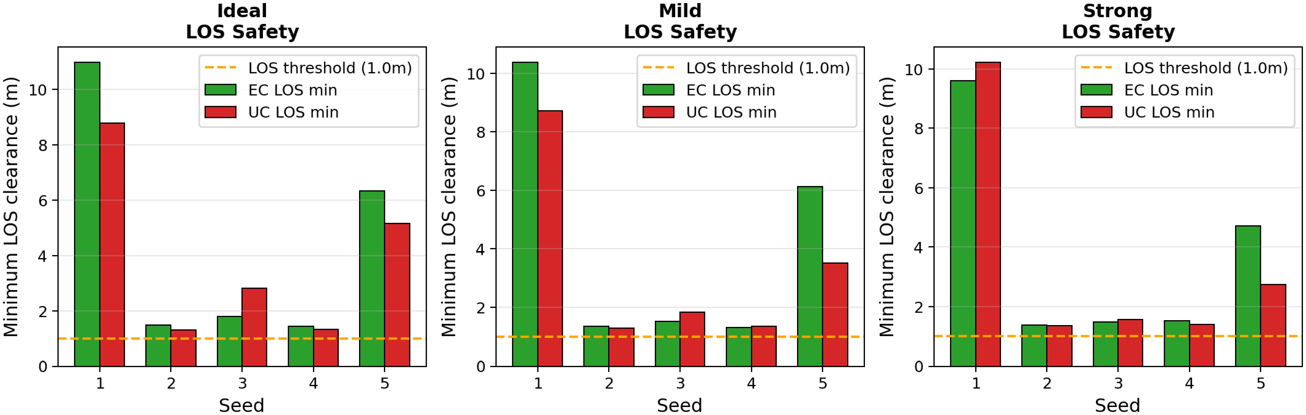
Figure 11. 

Minimum LOS clearance under ideal, mild-disturbance, and strong-disturbance execution. The dashed line denotes the LOS safety threshold of 1.0 m.

Figure 11 shows that both methods maintain LOS safety, with the minimum LOS clearance remaining above the $ 1.0\,{\rm{m}} $ threshold in all tested cases. These results indicate that the proposed energy-aware shielded execution retains its propulsion-energy advantage while preserving LOS feasibility under disturbance-aware simulation. Nevertheless, this remains a motion-level validation under the adopted propulsion-power surrogate, and the exact energy-saving percentage should not be interpreted as guaranteed real-flight power saving.

Propulsion energy model comparison

This experiment compares three embedded propulsion-energy models under identical task settings and constraint-consistent execution. We evaluate our model, denoted as Proposed, against two representative baselines. The task specification, obstacle field, UGV reference trajectory, motion limits, and feasibility checks are identical across methods. At each step, the controller produces a nominal UAV velocity command $ {\bf{v}}_{{\rm{des}},t} $, which is mapped by the Shield into the executed velocity $ {\bf{v}}_{{\rm{safe}},t} $. Propulsion energy is always computed from $ {\bf{v}}_{{\rm{safe}},t} $.

Let $ {\bf{v}}_{{\rm{safe}},t}=[{\bf{v}}_{xy,t}; v_{z,t}] $ denote the executed UAV velocity, with horizontal speed $ V_t=\|{\bf{v}}_{xy,t}\|_2 $. All methods share the same per-step energy structure:

The vertical power and total step-wise energy are:

All physical parameters are shared across models. The only difference is the definition of $ \kappa_t $.

The Proposed model uses:

Gao et al.^[34] increase $ \kappa_t $ according to the horizontal acceleration magnitude:

Yang et al.^[35] further couple acceleration and speed through an equivalent drag term:

where, m is the vehicle mass, g is the gravitational acceleration, and $ A_{{\rm{eq}}} $ is the equivalent frontal-area parameter.

To reduce bias from different completion distances, cumulative energy is aligned by UAV trajectory arc length:

We also report energy per distance $ E_{{\rm{ep}}}/D $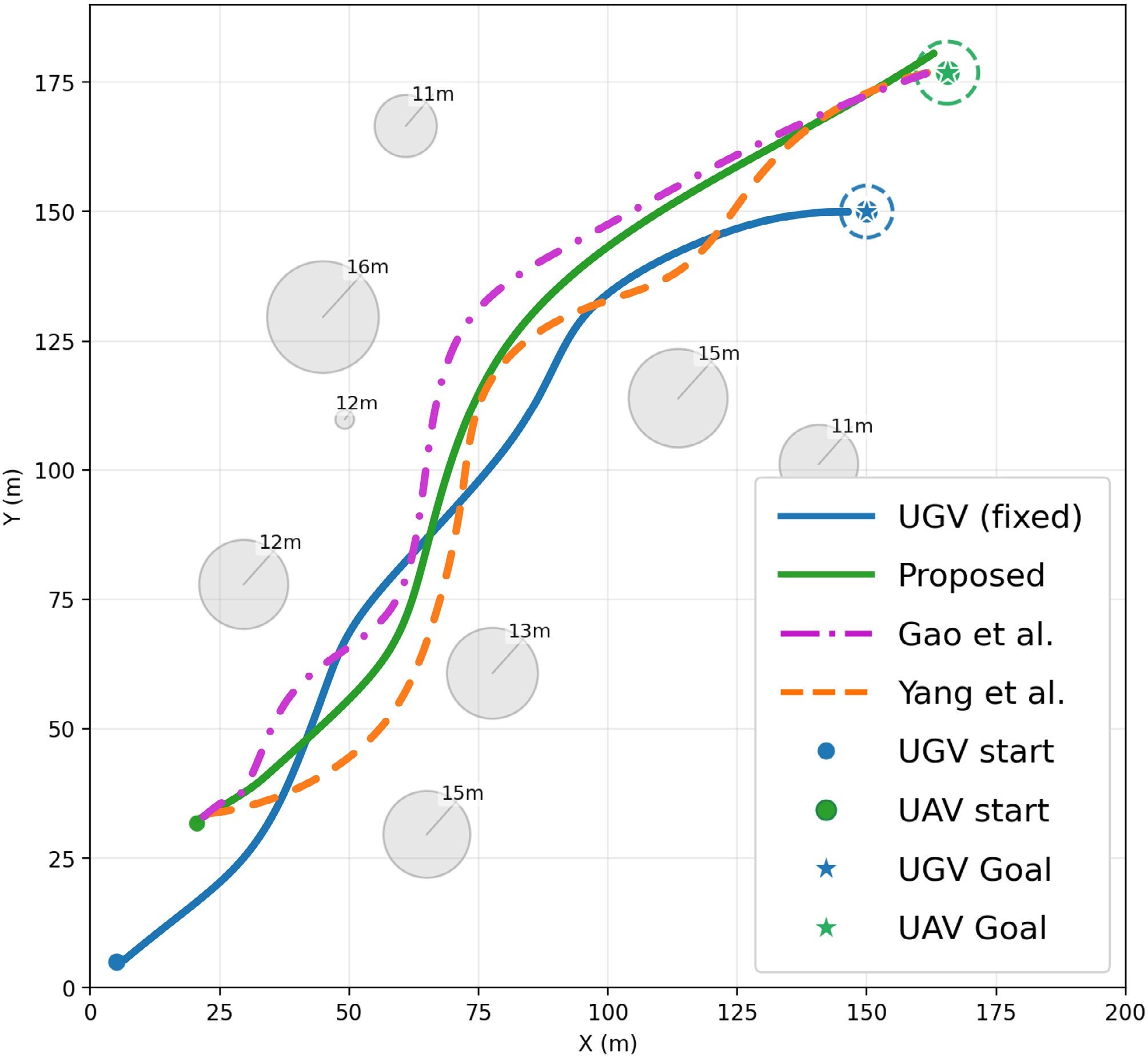, where D is the executed travel distance. The planar trajectories of the three methods are shown in Fig. 12.

Figure 12. 

Planar trajectories in the shared obstacle field. The UGV trajectory is fixed and shared. The three UAV trajectories correspond to proposed, Gao et al.^[34], and Yang et al.^[35]

The kinematic traces in Fig. 12 are consistent with the energy outcomes. All methods complete obstacle avoidance and forward tracking, while Proposed follows a more compact route and travels the shortest distance. The progress-aligned cumulative energy and instantaneous power are shown in Fig. 13.

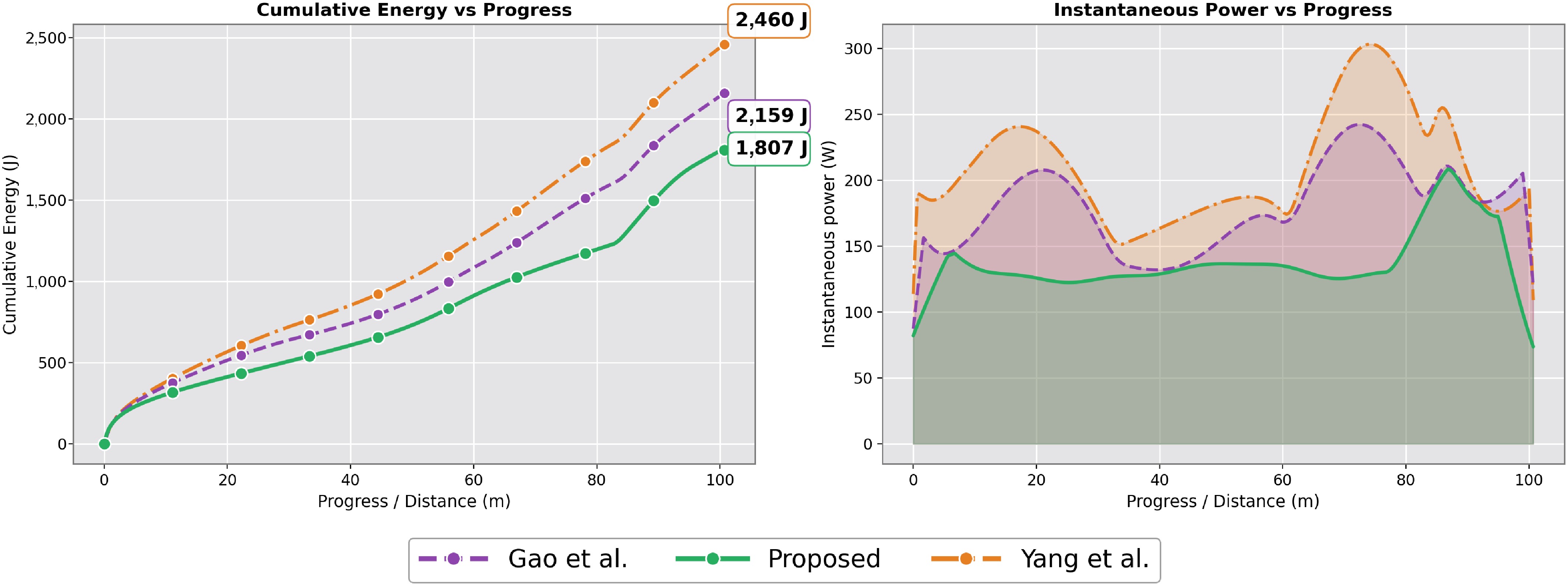
Figure 13. 

Progress-aligned cumulative energy and instantaneous power. Cumulative energy is compared at matched UAV progress to reduce bias from different travel distances.

Figure 13 shows that Proposed has the lowest progress-aligned cumulative energy and fewer high-power peaks. The LOS margin comparison is shown in Fig. 14.

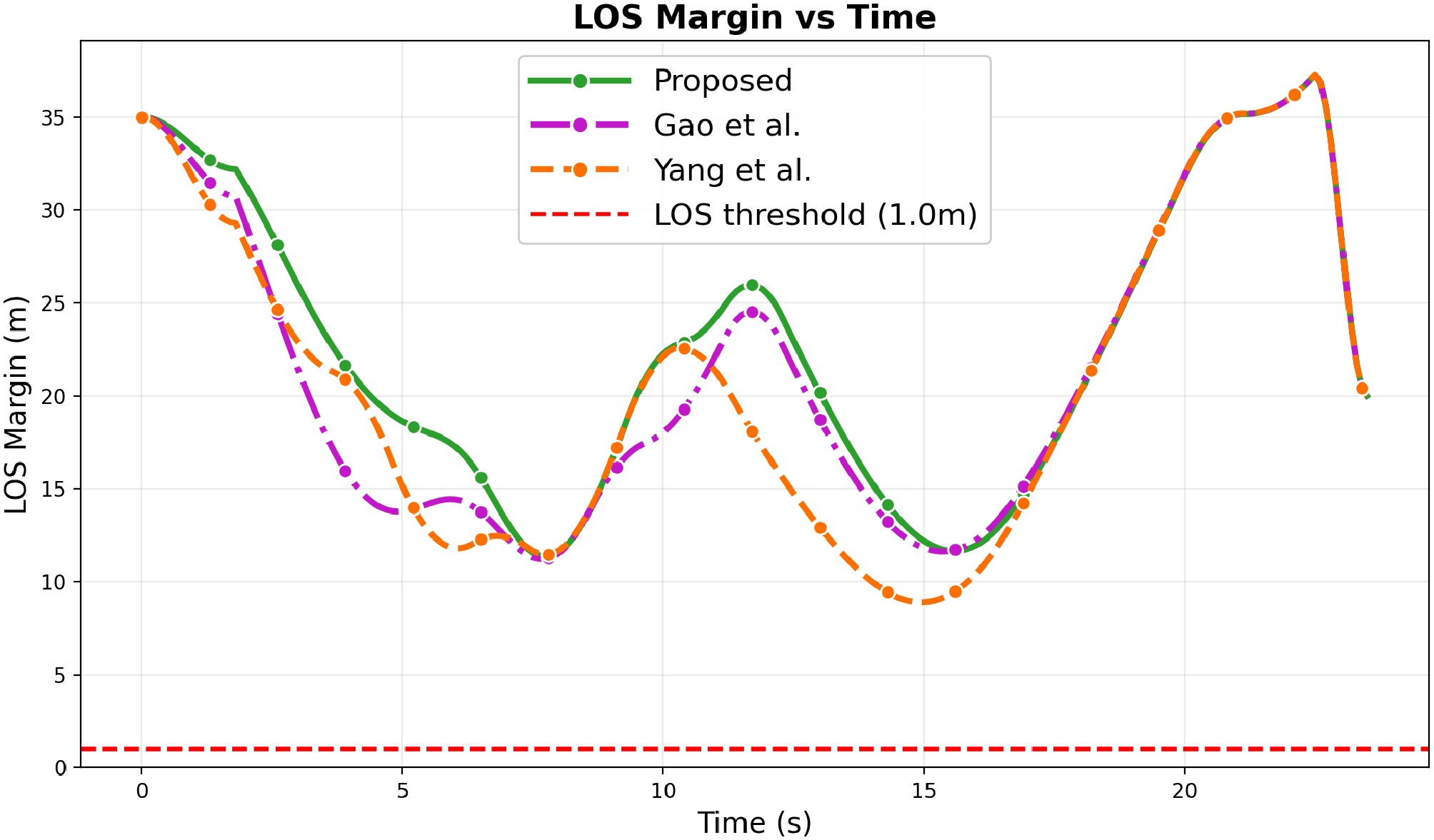
Figure 14. 

LOS margin over time under the three embedded propulsion-energy models, with $ \varepsilon_{\rm{LOS}}=1.0\rm{\ m} $.

Figure 14 shows that all three methods keep the LOS margin above $ \varepsilon_{{\rm{LOS}}}=1.0\,{\rm{m}} $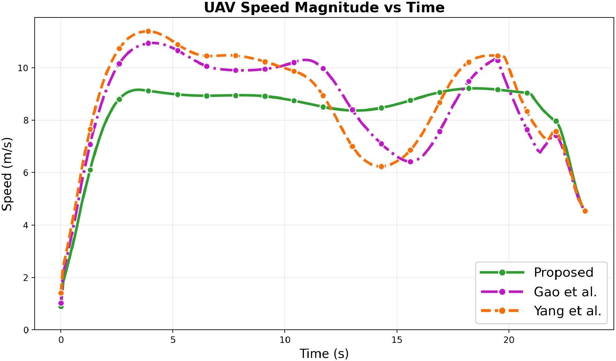, indicating that the energy differences are not obtained by approaching the LOS constraint. The speed profiles are shown in Fig. 15.

Figure 15. 

UAV speed magnitude over time under the three embedded propulsion-energy models.

Figure 15 further shows that Proposed maintains a lower and smoother speed profile, reducing operation in the high-speed region where the parasitic term $ P_3(V)\propto V^3 $ dominates. The slightly lower mean altitude of Proposed also reduces the vertical contribution under the shared vertical-power surrogate. The quantitative comparison is summarized in Table 2.

As reported in Table 2, Proposed reduces total energy by 16.3% and 26.5% compared with Gao et al. and Yang et al., respectively.

Overall, this comparison indicates that the proposed SAC–Shield design remains energy-efficient under different embedded propulsion-energy formulations, although absolute energy values may change with a higher-fidelity vehicle-calibrated power model.

Online runtime evaluation

To examine practical online performance, we profile the execution stage after training. The sampling period is $ \Delta t=0.1 $ s. The default setting uses $ N=15 $ local obstacles and $ S=64 $ LOS samples, consistent with Table 1. The controller is evaluated over 2,000 online control steps. The timing breakdown is reported in Table 3.

As reported in Table 3, the complete online control loop requires $ 33.60\pm7.56 $ ms per step on average, corresponding to approximately $ 29.8 $ Hz. The 95^th-percentile runtime is $ 46.76 $ ms, which remains below the $ 100 $ ms control period. The dominant components are LOS evaluation, candidate-direction search, and Shield mapping, which is consistent with the complexity analysis presented earlier. The scalability result with respect to local obstacles and LOS samples is shown in Table 4. Table 4 shows that the feasibility-evaluation time increases with N and S, following the expected $ O(KNS) $ trend. Even under the largest tested setting, the mean evaluation time remains below $ 100 $ ms. In practice, the computational load can be further bounded by considering local obstacles, using fixed LOS sampling density, or applying adaptive LOS sampling near potential occlusions.

The proposed framework provides an online motion-level correction mechanism for perceived geometric changes. At each control step, the Shield reconstructs the admissible velocity set using the latest UAV–UGV states, obstacle information, and LOS geometry. Thus, newly detected obstacles or updated LOS conditions can affect the executed command at the next control step.

The current study focuses on geometric feasibility and motion-level propulsion-energy evaluation. Network congestion, packet loss, bandwidth variation, dynamic-obstacle prediction, and detailed communication-network effects are not explicitly modeled. Therefore, the reported robustness should be interpreted as motion-level and visibility-level robustness rather than full communication-network robustness.

Moreover, the propulsion-energy metric used in this work is based on an executed-velocity-driven surrogate model. Physical flight tests, actual onboard power or battery-discharge measurements, high-fidelity hardware-in-the-loop validation, nonlinear battery dynamics, state-of-charge estimation, and high-fidelity motor-propeller modeling are outside the scope of the present work. Accordingly, the reported energy reductions should be interpreted as simulation-based motion-level estimates rather than calibrated real-world battery-saving measurements.

For long-duration deployment, the online energy estimate could be connected to a supervisory battery-management layer in future work. The remaining usable energy can be monitored by $ E_{{\rm{rem}},t}=E_{{\rm{bat}}}^{{\rm{use}}}-\sum_{\ell=0}^{t}E_{\ell} $, where $ E_{{\rm{bat}}}^{{\rm{use}}} $ is the usable onboard battery energy. When $ E_{{\rm{rem}},t} $ approaches a critical threshold, the supervisor could increase the energy weight, reduce velocity bounds, or switch the UAV to a rendezvous or return mode, while the Shield continues applying the sampled feasibility checks considered in this work. Future work will investigate real flight tests, actual onboard power measurements, high-fidelity hardware-in-the-loop validation, platform-specific power calibration, nonlinear battery modeling, high-fidelity motor-propeller modeling, and communication-aware planning.

This paper proposes an energy-efficient and constraint-consistent UAV–UGV control framework for forward reconnaissance under LOS maintenance constraints. A SAC policy generates nominal velocity commands, and the Shield maps them to feasible executed velocities. The executed velocity is used consistently for state propagation, energy accounting, reward evaluation, and feasibility checking.

Simulation results based on the adopted motion-level propulsion-energy surrogate show that the proposed method reduces estimated UAV propulsion energy while supporting sampled LOS feasibility and obstacle-avoidance feasibility in the tested scenarios. The inactive-constraint experiment verifies that the energy reduction mainly comes from learned speed scheduling rather than excessive Shield intervention. The propulsion-energy ablation confirms the benefit of including energy cost in the learning objective. The disturbance-aware validation shows that the estimated energy-saving trend remains positive under command delay, velocity-response lag, and wind disturbance in simulation. The propulsion-model comparison and runtime evaluation further indicate that the proposed SAC–Shield design retains a lower estimated propulsion-energy trend under different embedded energy formulations and is computationally tractable for online execution.

Future work will extend the framework to multi-UAV relay selection, multi-UGV task allocation, physical flight tests with actual onboard power measurements, high-fidelity hardware-in-the-loop validation, nonlinear battery dynamics and state-of-charge estimation, high-fidelity motor-propeller modeling, and fleet-level energy-aware coordination.