











-
Aerial manipulators are multirotor platforms equipped with one or more on-board robotic arms. They have emerged as a versatile means to extend the agility and reach of unmanned aerial vehicles from passive sensing toward active physical interaction with the environment[1,2]. Representative mission profiles include contact-based non-destructive testing (NDT) and tapping inspection on industrial structures, push-and-slide inspection of vertical surfaces, aerial sample collection, and aerial assembly[3]. A central challenge across these missions is the execution of contact operations against target surfaces whose material properties cannot be characterised prior to deployment. With the multirotor base typically stabilised in hover by its onboard flight controller (a cascaded attitude–position autopilot), the principal difficulty reduces to active regulation of the manipulator–environment interaction in the presence of unknown and possibly nonlinear contact dynamics. This is a key enabler of autonomous control for intelligent aerial vehicles operating in unstructured environments.
Impedance control, originally proposed by Hogan[4], addresses this difficulty by regulating the dynamic relationship between the contact force and the end-effector displacement instead of regulating either signal directly. The paradigm has been widely adopted in robotic interaction tasks[5,6] and extended to aerial manipulation. However, the impedance gains that determine the closed-loop compliance are difficult to choose without prior knowledge of the contact dynamics, motivating adaptive impedance control schemes that adjust the gains online from the observed interaction[7−9]. Early adaptive schemes used gradient-based update laws or model-reference structures that require either an explicit contact-model parameterisation or strong structural assumptions on the uncertainty; more recently, impedance-filter and vision-guided designs have been developed for time-varying contact-force regulation of aerial manipulators under uncertain physical interaction[10].
The contact model itself is a key but often understated element of these formulations. Most existing adaptive impedance methods adopt a linear spring–damper (Kelvin–Voigt) representation,
$ f_{c,n}=K\delta+c\dot\delta $ $ f_{c,n}=k_{c}\delta^{n_{p}}(1+b_{c}\dot\delta) $ $ n_{p}=3/2 $ Reinforcement learning (RL) has emerged as a powerful paradigm for solving optimal control problems in a model-free manner[14,15]. Integral reinforcement learning (IRL)[16,17] is particularly attractive for continuous-time systems with partially unknown drift, because it reformulates the Bellman equation as an integral condition along measured trajectories, thereby avoiding any explicit system identification step. Off-policy variants further decouple the data-collection policy from the policy being evaluated[17,18], enhancing data efficiency and removing the requirement of a known stabilising initial controller. Recent online off-policy RL methods recover optimal feedback for completely unknown continuous-time nonlinear plants from measured data alone[19]. Actor–Critic architectures, in which a Critic approximates the value function and an Actor represents the control policy, have proven effective for implementing IRL in continuous-time nonlinear settings[15,20]. Beyond the classical continuous-time setting, recent adaptive dynamic programming (ADP) results have broadened the class of plants for which a model-free optimal policy can be recovered online. Estimator-augmented ADP designs recover real-time optimal attitude and pose tracking for spacecraft under actuator misalignment, pointing constraints, and unknown dynamics[21,22], showing that an Actor–Critic loop can absorb substantial plant uncertainty without an identified plant model. On the algorithmic side, Hamiltonian-driven ADP accounts for approximation errors in the value-function residual[23], model-free
$ \lambda $ These observations expose a methodological gap. Designs that commit to a linear-contact assumption are tractable but suffer the modelling deficiencies above; designs that commit to a specific nonlinear parameterisation (such as the HC model with known
$ k_{c}, n_{p}, b_{c} $ This paper develops such a synthesis route. We adopt a single-loop direct Cartesian impedance realisation under which the closed-loop dynamics satisfy the prescribed impedance relation as an exact identity, separating the realisation of compliant behaviour—handled by a standard inverse-dynamics controller—from the design of the impedance gains, which is the focus of the paper. The principal contributions are as follows:
1. A contact-frame impedance formulation that projects the six-dimensional Cartesian impedance equation onto the contact frame and decomposes it into normal and tangential channels. The tangential channels are shown, via a direct specialization of standard input-to-state stability (ISS) results, to remain well-behaved under the baseline impedance and Coulomb friction without dedicated adaptation, so the design effort is restricted to the dominant normal direction.
2. An optimal-control reformulation in which the desired stiffness and damping along the normal direction are taken as virtual control inputs. The resulting Hamilton–Jacobi–Bellman equation isolates the unknown contact dynamics into the drift and leaves the input matrix and exogenous term exactly known, so a model-free Actor–Critic solution is feasible without committing to a specific contact-model parameterisation.
3. An off-policy integral reinforcement learning algorithm that solves the resulting optimal-control problem online from measured trajectory data. The same algorithmic data flow accommodates systems with partially unknown drift and fixed exogenous inputs, and a numerical study sweeps a parameterised family of nonlinear contact models to show that the proposed design retains tight contact-force tracking across the family, while a sample-based linear-quadratic alternative degrades by orders of magnitude as the contact nonlinearity grows.
The "Problem formulation" section develops the contact-frame projection and the resulting scalar normal-direction subproblem, treating the contact dynamics as an unspecified smooth function of indentation and indentation rate. The "Optimal control formulation of the adaptive impedance problem" section reformulates the subproblem as a nonlinear optimal-control problem and derives the associated HJB equation. The "Off-policy integral reinforcement learning algorithm" section develops the off-policy IRL algorithm that solves it. The "Numerical simulation" section reports the simulation studies on a Hunt–Crossley test contact, including the comparison with the sample-based linear-quadratic baseline, and the "Conclusions" section concludes.
-
A central challenge across these missions is the execution of contact operations against target surfaces whose material properties cannot be characterised prior to deployment, as illustrated in Fig. 1. The proposed framework is depicted in Fig. 2. The lower region implements a Cartesian impedance relation between the end-effector pose error and the contact wrench through inverse-dynamics torque commands; the upper region adapts the impedance gains on-line via off-policy integral reinforcement learning (IRL), constructed in the "Optimal control formulation of the adaptive impedance problem" and "Off-policy integral reinforcement learning algorithm" sections. Operation proceeds through three sequentially activated phases that recur throughout the paper. In the Approach phase, the manipulator transits to the contact surface under a fixed-gain baseline impedance, with no contact force and no learning. The Data-Collection phase begins at first contact: the baseline impedance remains in command, exploration noise is injected into the virtual control to ensure persistent excitation, and the resulting input–state trajectories are accumulated as off-policy training data. The Applied Phase activates the converged Actor–Critic pair, so that the learned policy generates the impedance gains in real time. The transitions Approach
$ \to $ $ \to $ 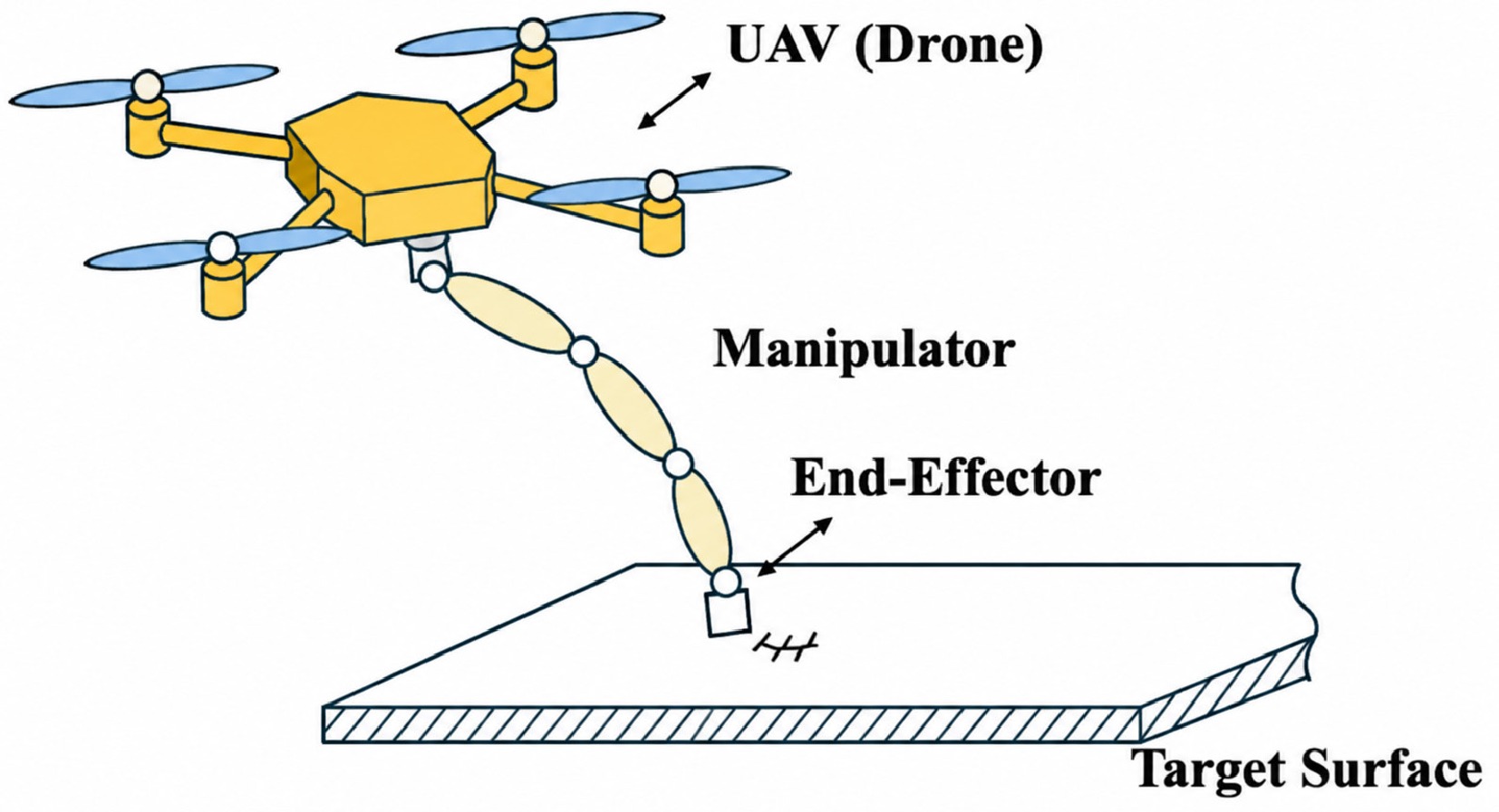
Figure 1.
Aerial manipulator performing contact-based surface interaction.
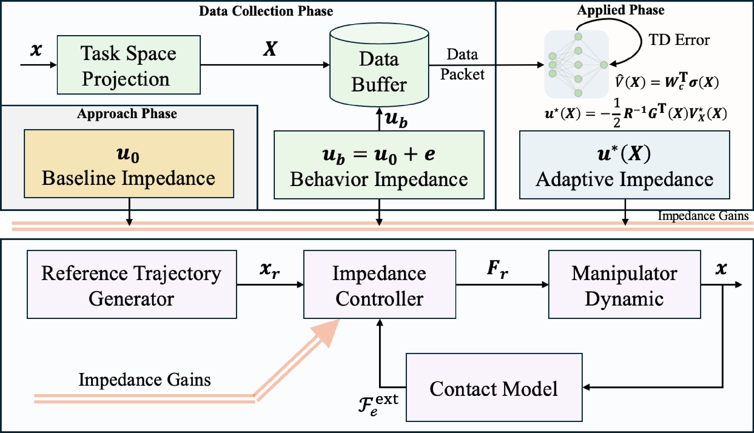
Figure 2.
Optimal adaptive impedance control framework.
Consider an aerial manipulator consisting of an
$ n $ $ {\boldsymbol{x}}_b \in \mathbb{R}^{6} $ $ {\boldsymbol{\theta}} \in \mathbb{R}^{n} $ $ {\boldsymbol{q}} = [{\boldsymbol{x}}_b^{\mathrm{T}},{\boldsymbol{\theta}}^{\mathrm{T}}]^{\mathrm{T}} \in \mathbb{R}^{n+6} $ $ \begin{array}{l} {\boldsymbol{M}}({\boldsymbol{q}})\ddot{{\boldsymbol{q}}} + {\boldsymbol{C}}({\boldsymbol{q}},\dot{{\boldsymbol{q}}})\dot{{\boldsymbol{q}}} + {\boldsymbol{G}}({\boldsymbol{q}}) \;=\; {\boldsymbol{\tau}}_{g} + {\boldsymbol{J}}_{e}^{\mathrm{T}}({\boldsymbol{q}})\,{\boldsymbol{\mathcal{F}}}_{e}^{\mathrm{ext}}, \end{array} $ (1) where,
$ {\boldsymbol{M}}({\boldsymbol{q}}) \in \mathbb{R}^{(n+6)\times(n+6)} $ $ {\boldsymbol{C}}({\boldsymbol{q}},\dot{{\boldsymbol{q}}}) $ $ {\boldsymbol{G}}({\boldsymbol{q}})\in\mathbb{R}^{n+6} $ $ {\boldsymbol{\tau}}_{g} = [{\boldsymbol{\mathcal{F}}}_b^{\mathrm{T}},\,{\boldsymbol{\tau}}^{\mathrm{T}}]^{\mathrm{T}} $ $ {\boldsymbol{\mathcal{F}}}_b \in \mathbb{R}^6 $ $ {\boldsymbol{\tau}} \in \mathbb{R}^n $ $ {\boldsymbol{\mathcal{F}}}_{e}^{\mathrm{ext}} \in \mathbb{R}^{6} $ $ {\boldsymbol{M}} $ $ {\boldsymbol{C}} $ $ {\boldsymbol{G}} $ $ {\boldsymbol{q}} $ $ \begin{array}{l} \begin{bmatrix} {\boldsymbol{M}}_{b} & {\boldsymbol{M}}_{bm} \\ {\boldsymbol{M}}_{bm}^{\mathrm{T}} & {\boldsymbol{M}}_{m} \end{bmatrix} \begin{bmatrix} \ddot{{\boldsymbol{x}}}_{b} \\ \ddot{{\boldsymbol{\theta}}} \end{bmatrix} + \begin{bmatrix} {\boldsymbol{C}}_{b} & {\boldsymbol{C}}_{bm} \\ {\boldsymbol{C}}_{mb} & {\boldsymbol{C}}_{m} \end{bmatrix} \begin{bmatrix} \dot{{\boldsymbol{x}}}_{b} \\ \dot{{\boldsymbol{\theta}}} \end{bmatrix} + \begin{bmatrix} {\boldsymbol{G}}_{b}({\boldsymbol{x}}_{b}) \\ {\boldsymbol{g}}_{m}({\boldsymbol{\theta}}) \end{bmatrix} \;=\; \begin{bmatrix} {\boldsymbol{\mathcal{F}}}_{b} \\ {\boldsymbol{\tau}} \end{bmatrix} + \begin{bmatrix} {\boldsymbol{J}}_{b}^{\mathrm{T}} \\ {\boldsymbol{J}}_{m}^{\mathrm{T}} \end{bmatrix}{\boldsymbol{\mathcal{F}}}_{e}^{\mathrm{ext}}, \end{array} $ (2) where,
$ {\boldsymbol{J}}_{b} \in \mathbb{R}^{6\times 6} $ $ {\boldsymbol{J}}_{m} \in \mathbb{R}^{6\times n} $ $ {\boldsymbol{J}}_{e}=[{\boldsymbol{J}}_{b},\,{\boldsymbol{J}}_{m}] $ $ \dot{{\boldsymbol{q}}} $ $ \dot{{\boldsymbol{x}}} $ $ {\boldsymbol{x}}\in\mathbb{R}^{6} $ $ \begin{array}{l} \dot{{\boldsymbol{x}}} \;=\; {\boldsymbol{J}}_{e}\dot{{\boldsymbol{q}}} \;=\; {\boldsymbol{J}}_{b}\dot{{\boldsymbol{x}}}_{b} + {\boldsymbol{J}}_{m}\dot{{\boldsymbol{\theta}}}. \end{array} $ (3) The off-diagonal block couplings
$ {\boldsymbol{M}}_{bm}\ddot{{\boldsymbol{\theta}}} $ $ {\boldsymbol{C}}_{bm}\dot{{\boldsymbol{\theta}}} $ $ {\boldsymbol{G}}_{b}({\boldsymbol{x}}_{b}) $ $ {\boldsymbol{\mathcal{F}}}_{e}^{\mathrm{ext}} $ $ {\boldsymbol{J}}_{b} $ $ {\boldsymbol{J}}_{m} $ Assumption 1 (Independently stabilised base) The multirotor base is independently and actively stabilised by its onboard flight controller such that, on the time scale of the contact event,
$ {\boldsymbol{x}}_b $ $ \dot{{\boldsymbol{x}}}_b \approx {\boldsymbol{0}} $ $ \ddot{{\boldsymbol{x}}}_b \approx {\boldsymbol{0}} $ Remark 1 Assumption 1 is directly satisfied by fully-actuated multirotor platforms (e.g., tilted-rotor hexa- or octocopters) that can apply an arbitrary six-DOF base wrench
$ {\boldsymbol{\mathcal{F}}}_{b} $ $ \dot{{\boldsymbol{x}}}_{b}\approx\ddot{{\boldsymbol{x}}}_{b}\approx{\boldsymbol{0}} $ Under Assumption 1, Eqs (2) and (3) are reduced to
$ \begin{array}{l} \left\{ \begin{aligned} &{\boldsymbol{M}}_{m}({\boldsymbol{\theta}})\ddot{{\boldsymbol{\theta}}} + {\boldsymbol{C}}_{m}({\boldsymbol{\theta}},\dot{{\boldsymbol{\theta}}})\dot{{\boldsymbol{\theta}}} + {\boldsymbol{g}}_{m}({\boldsymbol{\theta}}) = {\boldsymbol{\tau}} + {\boldsymbol{J}}_{m}^{\mathrm{T}}({\boldsymbol{\theta}})\,{\boldsymbol{\mathcal{F}}}_{e}^{\mathrm{ext}}, \\ &\dot{{\boldsymbol{x}}} = {\boldsymbol{J}}_{m}({\boldsymbol{\theta}})\,\dot{{\boldsymbol{\theta}}}, \\ &\ddot{{\boldsymbol{x}}} = {\boldsymbol{J}}_{m}({\boldsymbol{\theta}})\,\ddot{{\boldsymbol{\theta}}} + \dot{{\boldsymbol{J}}}_{m}({\boldsymbol{\theta}})\,\dot{{\boldsymbol{\theta}}}. \end{aligned} \right. \end{array} $ (4) Provided that
$ {\boldsymbol{J}}_{m} $ $ \begin{array}{l} \bar{{\boldsymbol{M}}}({\boldsymbol{\theta}})\ddot{{\boldsymbol{x}}} + \bar{{\boldsymbol{C}}}({\boldsymbol{\theta}},\dot{{\boldsymbol{\theta}}})\dot{{\boldsymbol{x}}} + \bar{{\boldsymbol{g}}}({\boldsymbol{\theta}}) \;=\; {\boldsymbol{F}}_{\tau} + {\boldsymbol{\mathcal{F}}}_{e}^{\mathrm{ext}}, \end{array} $ (5) with
$ \bar{{\boldsymbol{M}}}({\boldsymbol{\theta}}) = {\boldsymbol{J}}_{m}^{-\mathrm{T}}{\boldsymbol{M}}_{m}{\boldsymbol{J}}_{m}^{-1} $ $ \bar{{\boldsymbol{C}}} $ $ \bar{{\boldsymbol{g}}}({\boldsymbol{\theta}})={\boldsymbol{J}}_{m}^{-\mathrm{T}}{\boldsymbol{g}}_{m}({\boldsymbol{\theta}}) $ $ {\boldsymbol{F}}_{\tau} = {\boldsymbol{J}}_{m}^{-\mathrm{T}}{\boldsymbol{\tau}} $ Compliant interaction is enforced through a desired second-order impedance relation. Let
$ {\boldsymbol{x}}_{r}(t)\in\mathbb{R}^{6} $ $ \tilde{{\boldsymbol{x}}}={\boldsymbol{x}}-{\boldsymbol{x}}_{r}\in\mathbb{R}^{6} $ $ {\boldsymbol{F}}_{d}\in\mathbb{R}^{6} $ $ \begin{array}{l} {\boldsymbol{M}}_{d}\ddot{\tilde{{\boldsymbol{x}}}} + {\boldsymbol{D}}_{d}\dot{\tilde{{\boldsymbol{x}}}} + {\boldsymbol{K}}_{d}\tilde{{\boldsymbol{x}}} \;=\; {\boldsymbol{\mathcal{F}}}_{e}^{\mathrm{ext}} - {\boldsymbol{F}}_{d}, \end{array} $ (6) where,
$ {\boldsymbol{M}}_{d},{\boldsymbol{D}}_{d},{\boldsymbol{K}}_{d}\in\mathbb{R}^{6\times 6} $ $ {\boldsymbol{\mathcal{F}}}_{e}^{\mathrm{ext}} $ $ \begin{array}{l} {\boldsymbol{F}}_{\tau} \;=\;\bar{{\boldsymbol{M}}}({\boldsymbol{\theta}})\Bigl[\ddot{{\boldsymbol{x}}}_{r}-{\boldsymbol{M}}_{d}^{-1}\bigl({\boldsymbol{D}}_{d}\dot{\tilde{{\boldsymbol{x}}}}+{\boldsymbol{K}}_{d}\tilde{{\boldsymbol{x}}}-{\boldsymbol{\mathcal{F}}}_{e}^{\mathrm{ext}}+{\boldsymbol{F}}_{d}\bigr)\Bigr] +\bar{{\boldsymbol{C}}}({\boldsymbol{\theta}},\dot{{\boldsymbol{\theta}}})\dot{{\boldsymbol{x}}}+\bar{{\boldsymbol{g}}}({\boldsymbol{\theta}})-{\boldsymbol{\mathcal{F}}}_{e}^{\mathrm{ext}}, \end{array} $ (7) applied via
$ {\boldsymbol{\tau}}={\boldsymbol{J}}_{m}^{\mathrm{T}}({\boldsymbol{\theta}}){\boldsymbol{F}}_{\tau} $ $ \bar{{\boldsymbol{C}}}\dot{{\boldsymbol{x}}} $ $ \bar{{\boldsymbol{g}}} $ $ {\boldsymbol{\mathcal{F}}}_{e}^{\mathrm{ext}} $ $ \bar{{\boldsymbol{M}}}^{-1}{\boldsymbol{M}}_{d} $ $ (\bar{{\boldsymbol{M}}},\bar{{\boldsymbol{C}}},\bar{{\boldsymbol{g}}}) $ $ ({\boldsymbol{D}}_{d},{\boldsymbol{K}}_{d}) $ $ \bar{{\boldsymbol{g}}}({\boldsymbol{\theta}}) $ Remark 2 The controller (7) relies on the manipulator dynamics
$ (\bar{{\boldsymbol{M}}},\bar{{\boldsymbol{C}}},\bar{{\boldsymbol{g}}}) $ Taskspace projection of impedance control
-
The design Eq. (6) is six-dimensional, whereas the contact wrench in surface-contact tasks acts in a low-dimensional subspace aligned with the contact geometry. Direct adaptive synthesis in
$ \mathbb{R}^{6} $ The end-effector pose error is decomposed as
$ \tilde{{\boldsymbol{x}}}=[\tilde{{\boldsymbol{p}}}^{\mathrm{T}},\,\tilde{{\boldsymbol{\phi}}}^{\mathrm{T}}]^{\mathrm{T}} $ $ \tilde{{\boldsymbol{p}}} \in \mathbb{R}^{3} $ $ \tilde{{\boldsymbol{\phi}}} \in \mathbb{R}^{3} $ $ \begin{array}{l} {\boldsymbol{M}}_{d}=\mathrm{blkdiag}\bigl({\boldsymbol{M}}_{d}^{p},{\boldsymbol{M}}_{d}^{\phi}\bigr),\quad {\boldsymbol{D}}_{d}=\mathrm{blkdiag}\bigl({\boldsymbol{D}}_{d}^{p},{\boldsymbol{D}}_{d}^{\phi}\bigr),\quad {\boldsymbol{K}}_{d}=\mathrm{blkdiag}\bigl({\boldsymbol{K}}_{d}^{p},{\boldsymbol{K}}_{d}^{\phi}\bigr), \end{array} $ (8) which separates translational and rotational impedance loops. The surface-contact tasks considered here are governed by the following geometric premise on the contact.
Assumption 2 (Contact-surface geometry) For the surface-contact tasks considered in this paper: (a) the contact wrench carries no moment about the end-effector, acting only as a force in the tangent plane and along the surface normal; and (b) the outward surface normal is locally constant over the contact arc swept during the task, so that the contact frame
$ \{{\boldsymbol{n}},{\boldsymbol{t}}_{1},{\boldsymbol{t}}_{2}\} $ $ {\boldsymbol{B}} $ By Assumption 2(a), the contact wrench carries no contact moment, so the rotational sub-equation reduces to the linear regulator
$ {\boldsymbol{M}}_{d}^{\phi}\ddot{\tilde{{\boldsymbol{\phi}}}}+{\boldsymbol{D}}_{d}^{\phi}\dot{\tilde{{\boldsymbol{\phi}}}}+{\boldsymbol{K}}_{d}^{\phi}\tilde{{\boldsymbol{\phi}}}=-{\boldsymbol{m}}_{d} $ $ {\boldsymbol{m}}_{d} $ $ {\boldsymbol{F}}_{d} $ $ {\boldsymbol{x}}_{r}\in\mathbb{R}^{3} $ $ \tilde{{\boldsymbol{p}}}={\boldsymbol{p}}-{\boldsymbol{x}}_{r} $ $ \begin{array}{l} {\boldsymbol{M}}_{d}^{p}\ddot{\tilde{{\boldsymbol{p}}}} + {\boldsymbol{D}}_{d}^{p}\dot{\tilde{{\boldsymbol{p}}}} + {\boldsymbol{K}}_{d}^{p}\tilde{{\boldsymbol{p}}} \;=\; {\boldsymbol{f}}_{c} - {\boldsymbol{f}}_{d}, \end{array} $ (9) where,
$ {\boldsymbol{f}}_{c} \in \mathbb{R}^{3} $ $ {\boldsymbol{\mathcal{F}}}_{e}^{\mathrm{ext}} $ $ {\boldsymbol{f}}_{d} \in \mathbb{R}^{3} $ $ {\boldsymbol{F}}_{d} $ Let
$ \{{\boldsymbol{n}},{\boldsymbol{t}}_{1},{\boldsymbol{t}}_{2}\}\subset\mathbb{R}^{3} $ $ {\boldsymbol{n}} $ $ {\boldsymbol{t}}_{1},{\boldsymbol{t}}_{2} $ $ \begin{array}{l} {\boldsymbol{B}} \;=\; \bigl[{\boldsymbol{n}}\;\,{\boldsymbol{t}}_{1}\;\,{\boldsymbol{t}}_{2}\bigr]\in\mathbb{R}^{3\times 3}, \qquad {\boldsymbol{B}}^{\mathrm{T}}{\boldsymbol{B}}={\boldsymbol{I}}_{3}. \end{array} $ (10) Following standard task-frame impedance design[5,6], the translational impedance matrices are taken as diagonal in this contact frame, i.e., the user prescribes independent compliance along the normal and the two tangential directions:
$ \begin{array}{l} \left\{ \begin{aligned} {\boldsymbol{B}}^{\mathrm{T}} {\boldsymbol{M}}_{d}^{p} {\boldsymbol{B}} &= \mathrm{diag}(M_n,\, M_{t_1},\, M_{t_2}), \\ {\boldsymbol{B}}^{\mathrm{T}} {\boldsymbol{D}}_{d}^{p} {\boldsymbol{B}} &= \mathrm{diag}(D_n,\, D_{t_1},\, D_{t_2}), \\ {\boldsymbol{B}}^{\mathrm{T}} {\boldsymbol{K}}_{d}^{p} {\boldsymbol{B}} &= \mathrm{diag}(K_n,\, K_{t_1},\, K_{t_2}). \end{aligned} \right. \end{array} $ (11) Let the projected coordinates be defined as
$ \tilde{p}_{i}={\boldsymbol{e}}_{i}^{\mathrm{T}}\tilde{{\boldsymbol{p}}} $ $ f_{c,i}={\boldsymbol{e}}_{i}^{\mathrm{T}}{\boldsymbol{f}}_{c} $ $ f_{d,i}={\boldsymbol{e}}_{i}^{\mathrm{T}}{\boldsymbol{f}}_{d} $ $ i\in\{n,t_{1},t_{2}\} $ $ {\boldsymbol{e}}_{n}={\boldsymbol{n}} $ $ {\boldsymbol{e}}_{t_{j}}={\boldsymbol{t}}_{j} $ $ {\boldsymbol{B}}^{\mathrm{T}}\tilde{{\boldsymbol{p}}}=[\tilde p_{n},\tilde p_{t_{1}},\tilde p_{t_{2}}]^{\mathrm{T}} $ $ {\boldsymbol{B}} $ $ {\boldsymbol{B}}^{\mathrm{T}} $ $ {\boldsymbol{B}}{\boldsymbol{B}}^{\mathrm{T}}={\boldsymbol{I}}_{3} $ $ {\boldsymbol{B}}^{\mathrm{T}}{\boldsymbol{M}}_{d}^{p} $ $ \ddot{\tilde{{\boldsymbol{p}}}} $ $ \begin{array}{l} M_{n}\ddot{\tilde p}_{n} + D_{n}\dot{\tilde p}_{n} + K_{n}\tilde p_{n} \;=\; f_{c,n} - f_{d,n}, \end{array} $ (12) $ \begin{array}{l} M_{t_{j}}\ddot{\tilde p}_{t_{j}} + D_{t_{j}}\dot{\tilde p}_{t_{j}} + K_{t_{j}}\tilde p_{t_{j}} \;=\; f_{c,t_{j}} - f_{d,t_{j}}, \qquad j=1,2. \end{array} $ (13) Equation (12) is generally nonlinear and parametrically uncertain:
$ f_{c,n}=g(\delta,\dot\delta) $ $ \delta=\tilde p_{n}+x_{r,n}-p_{e,n}\geq 0 $ $ p_{e,n}={\boldsymbol{n}}^{\mathrm{T}}{\boldsymbol{p}}_{e} $ $ f_{c,t_{j}}-f_{d,t_{j}} $ Property 1 (Reduction to a scalar normal subproblem) Under Assumption 2 and the block-diagonal design Eq. (8) together with the contact-frame diagonalization (11), the closed-loop Cartesian impedance Eq. (6) decomposes into (i) a rotational linear regulator, (ii) two tangential linear regulators (13), and (iii) a single scalar normal-direction regulator Eq. (12) into which all unknown contact nonlinearity is concentrated. The optimal adaptive impedance design therefore reduces, within the present modeling scope, to the synthesis of
$ (D_{n},K_{n}) $ Tangential channels under Coulomb friction
-
A natural concern raised by Property 1 is whether the tangential channels remain well-behaved when the contact-tangent force is non-zero. The most important physical mechanism that activates this concern is dry friction. Adopting the Coulomb friction model in the sliding regime,
$ \begin{array}{l} f_{c,t_{j}}(t) \;=\; -\mu\,f_{c,n}(t)\,\dfrac{\dot p_{t_{j}}(t)}{\|{\boldsymbol{v}}_{t}(t)\|},\qquad j=1,2,\quad \|{\boldsymbol{v}}_{t}\| \gt 0, \end{array} $ (14) with
$ \mu\in[0,\bar{\mu}] $ $ \bar{\mu}<\infty $ $ {\boldsymbol{v}}_{t}=[\dot p_{t_{1}},\dot p_{t_{2}}]^{\mathrm{T}} $ $ \dot p_{t_{j}}/\|{\boldsymbol{v}}_{t}\|\in[-1, 1] $ $ \begin{array}{l} |f_{c,t_{j}}(t)| \;\le\; \bar{\mu}\,|f_{c,n}(t)|. \end{array} $ (15) By substitution of (14) into (13) (with
$ f_{d,t_{j}}=0 $ $ \begin{array}{l} M_{t_{j}}\ddot{\tilde p}_{t_{j}} + D_{t_{j}}\dot{\tilde p}_{t_{j}} + K_{t_{j}}\tilde p_{t_{j}} \;=\; w_{j}(t),\qquad |w_{j}(t)|\le \bar{\mu}\,|f_{c,n}(t)|. \end{array} $ (16) The next proposition records the corresponding well-known stability properties; we state it explicitly because it underwrites the dimensional reduction of Property 1, but it claims no original mathematics—it is a direct specialization of the standard ISS results for Hurwitz LTI systems[26].
Proposition 1 (Specialization of standard ISS to the friction-driven tangential channel) For each
$ j\in\{1,2\} $ $ (M_{t_{j}},D_{t_{j}},K_{t_{j}}) $ $ f_{c,n} $ $ f_{c,n} \to f_{d,n} $ $ \dot x_{r,t_{j}}\equiv v_{0} \neq 0 $ $ \begin{array}{l} \bigl|\tilde p_{t_{j}}^{\,ss}\bigr| \;=\; \dfrac{\mu\,f_{d,n}}{K_{t_{j}}} \;\le\; \dfrac{\bar{\mu}\,f_{d,n}}{K_{t_{j}}}. \end{array} $ (17) Proof ISS follows from the
$ L^{\infty} $ $ \dot p_{t_{j}}/\|{\boldsymbol{v}}_{t}\|\to\mathrm{sign}(v_{0}) $ □ Remark 3 Proposition 1 converts the heuristic claim that the tangential channels need no learning into a quantitative statement: extending IRL to the tangent plane buys no stability margin, and the only price of not adapting is the bounded offset (17). Should this offset be unacceptable, feed-forwarding the measured
$ f_{c,t_{j}} $ $ \mu $ The remainder of the paper is dedicated to the synthesis problem identified by Property 1, namely the optimal adaptive design of
$ (D_{n},K_{n}) $ -
The virtual control input is defined as
$ \begin{array}{l} {\boldsymbol{u}} \;\triangleq\; \begin{bmatrix} D_{n} \\ K_{n} \end{bmatrix} \;\in\; \mathbb{R}^{2}. \end{array} $ (18) By substituting (18) into (12) and isolating
$ \ddot{\tilde p}_{n} $ $ \begin{array}{l} \ddot{\tilde p}_{n} \;=\; \dfrac{1}{M_{n}}\,f_{c,n}(\delta,\dot\delta) \;-\; \dfrac{1}{M_{n}}\,f_{d,n} \;-\; \dfrac{1}{M_{n}}\,\bigl[\,\dot{\tilde p}_{n},\;\tilde p_{n}\,\bigr]\,{\boldsymbol{u}}. \end{array} $ (19) Equation (19) reveals the structural property that drives the rest of the formulation: the gain–state products
$ D_{n}\dot{\tilde p}_{n} $ $ K_{n}\tilde p_{n} $ $ {\boldsymbol{u}} $ The reference signal
$ {\boldsymbol{x}}_{r}(t) $ $ \delta=\tilde p_{n}+x_{r,n}-p_{e,n} $ $ \dot\delta=\dot{\tilde p}_{n}+\dot x_{r,n} $ Assumption 3 (Linear command generator[27]) The translational reference trajectory
$ {\boldsymbol{x}}_{r}(t)\in\mathbb{R}^{p} $ $ p=3 $ $ \left\{\begin{array}{l} \dot{{\boldsymbol{\zeta}}} \;=\; {\boldsymbol{A}}_{d}\,{\boldsymbol{\zeta}} + {\boldsymbol{r}}_{d}, \\ {\boldsymbol{x}}_{r} \;=\; {\boldsymbol{C}}_{d}\,{\boldsymbol{\zeta}}, \end{array} \right. $ (20) where,
$ {\boldsymbol{\zeta}}\in\mathbb{R}^{q} $ $ {\boldsymbol{A}}_{d}\in\mathbb{R}^{q\times q} $ $ {\boldsymbol{C}}_{d}\in\mathbb{R}^{p\times q} $ $ {\boldsymbol{r}}_{d}\in\mathbb{R}^{q} $ Under Assumption 3,
$ \dot x_{r,n} = {\boldsymbol{n}}^{\mathrm{T}}{\boldsymbol{C}}_{d}\dot{{\boldsymbol{\zeta}}} = {\boldsymbol{n}}^{\mathrm{T}}{\boldsymbol{C}}_{d}\bigl({\boldsymbol{A}}_{d}{\boldsymbol{\zeta}}+{\boldsymbol{r}}_{d}\bigr) $ $ {\boldsymbol{\zeta}} $ $ {\boldsymbol{\zeta}} $ $ \begin{array}{l} {\boldsymbol{X}} \;=\; \bigl[\,\dot{\tilde p}_{n},\;\tilde p_{n},\;{\boldsymbol{\zeta}}^{\mathrm{T}}\,\bigr]^{\mathrm{T}} \;\in\; \mathbb{R}^{2+q}, \end{array} $ (21) under which both
$ x_{r,n}={\boldsymbol{n}}^{\mathrm{T}}{\boldsymbol{C}}_{d}{\boldsymbol{\zeta}} $ $ \dot x_{r,n} $ $ {\boldsymbol{X}} $ $ f_{c,n} $ $ f_{c,n}({\boldsymbol{X}}) $ $ \begin{array}{l} \dot{{\boldsymbol{X}}} \;=\; {\boldsymbol{F}}({\boldsymbol{X}}) \;+\; {\boldsymbol{G}}({\boldsymbol{X}})\,{\boldsymbol{u}} \;+\; {\boldsymbol{d}}, \end{array} $ (22) with
$ \begin{array}{l} {\boldsymbol{F}}({\boldsymbol{X}}) \;=\; \begin{bmatrix} M_{n}^{-1}\,f_{c,n}({\boldsymbol{X}}) \\ \dot{\tilde p}_{n} \\ {\boldsymbol{A}}_{d}\,{\boldsymbol{\zeta}} \end{bmatrix}, \quad {\boldsymbol{G}}({\boldsymbol{X}}) \;=\; -\dfrac{1}{M_{n}}\begin{bmatrix} \dot{\tilde p}_{n} & \tilde p_{n} \\ 0 & 0 \\ {\boldsymbol{0}}_{q\times 2} \end{bmatrix}, \quad {\boldsymbol{d}} \;=\; \begin{bmatrix} -M_{n}^{-1}\,f_{d,n} \\ 0 \\ {\boldsymbol{r}}_{d} \end{bmatrix}. \end{array} $ (23) Remark 4 Three structural features of (22) and (23) are essential for the developments that follow. (i) The unknown contact dynamics enter only the drift
$ {\boldsymbol{F}}({\boldsymbol{X}}) $ $ f_{c,n}({\boldsymbol{X}}) $ $ {\boldsymbol{G}}({\boldsymbol{X}}) $ $ {\boldsymbol{d}} $ $ {\boldsymbol{d}} $ $ f_{d,n} $ $ {\boldsymbol{r}}_{d} $ $ ({\boldsymbol{X}},{\boldsymbol{u}}) $ $ {\boldsymbol{G}}({\boldsymbol{X}}) $ $ {\boldsymbol{X}} $ $ {\boldsymbol{u}} $ $ {\boldsymbol{u}} $ HJB equation
-
To enforce simultaneous force tracking (
$ f_{c,n}\to f_{d,n} $ $ \tilde p_{n}\to 0 $ $ J({\boldsymbol{u}};{\boldsymbol{X}}(t)) \;=\; \int_{t}^{\infty} e^{-\alpha(\tau-t)}\, \bigl({\boldsymbol{X}}^{\mathrm{T}}(\tau){\boldsymbol{Q}}{\boldsymbol{X}}(\tau)+{\boldsymbol{u}}^{\mathrm{T}}(\tau){\boldsymbol{R}}\,{\boldsymbol{u}}(\tau)\bigr)\,d\tau, $ (24) where,
$ \alpha>0 $ $ {\boldsymbol{Q}}\in\mathbb{R}^{(2+q)\times(2+q)} $ $ {\boldsymbol{R}}\in\mathbb{R}^{2\times 2} $ $ {\boldsymbol{u}}=[D_{n},K_{n}]^{\mathrm{T}} $ $ {\boldsymbol{u}}^{\mathrm{T}}{\boldsymbol{R}}{\boldsymbol{u}} $ $ {\boldsymbol{R}} $ $ \alpha $ $ {\boldsymbol{d}} $ $ \alpha $ For notational economy, absorb the constant exogenous term into an augmented drift,
$ \tilde{{\boldsymbol{F}}}({\boldsymbol{X}}) \triangleq {\boldsymbol{F}}({\boldsymbol{X}})+{\boldsymbol{d}} $ $ \dot{{\boldsymbol{X}}}=\tilde{{\boldsymbol{F}}}({\boldsymbol{X}})+{\boldsymbol{G}}({\boldsymbol{X}}){\boldsymbol{u}} $ $ {\boldsymbol{V}}_{{\boldsymbol{X}}}\triangleq\partial V/\partial{\boldsymbol{X}} $ $ V({\boldsymbol{X}}) $ $ {\boldsymbol{V}}_{{\boldsymbol{X}}}^{\star} $ $ \hat{{\boldsymbol{V}}}_{{\boldsymbol{X}}} $ $ V^{\star}({\boldsymbol{X}})=\min_{{\boldsymbol{u}}}J({\boldsymbol{u}};{\boldsymbol{X}}) $ $ \begin{array}{l} \mathcal{H}({\boldsymbol{X}},V,{\boldsymbol{u}})\;=\;{\boldsymbol{X}}^{\mathrm{T}}{\boldsymbol{Q}}{\boldsymbol{X}}+{\boldsymbol{u}}^{\mathrm{T}}{\boldsymbol{R}}\,{\boldsymbol{u}}-\alpha V+{\boldsymbol{V}}_{{\boldsymbol{X}}}^{\mathrm{T}}\bigl(\tilde{{\boldsymbol{F}}}({\boldsymbol{X}})+{\boldsymbol{G}}({\boldsymbol{X}}){\boldsymbol{u}}\bigr). \end{array} $ (25) Since
$ {\boldsymbol{u}} $ $ {\boldsymbol{u}}^{\mathrm{T}}{\boldsymbol{R}}{\boldsymbol{u}} $ $ {\boldsymbol{V}}_{{\boldsymbol{X}}}^{\mathrm{T}}{\boldsymbol{G}}({\boldsymbol{X}}){\boldsymbol{u}} $ $ {\boldsymbol{u}} $ $ \dfrac{\partial\mathcal{H}}{\partial{\boldsymbol{u}}}\;=\;2{\boldsymbol{R}}\,{\boldsymbol{u}}\;+\;{\boldsymbol{G}}^{\mathrm{T}}({\boldsymbol{X}})\,{\boldsymbol{V}}_{{\boldsymbol{X}}}. $ Setting this gradient to
$ {\boldsymbol{0}} $ $ {\boldsymbol{u}} $ $ {\boldsymbol{u}}^{\star}({\boldsymbol{X}})\;=\;-\dfrac{1}{2}{\boldsymbol{R}}^{-1}{\boldsymbol{G}}^{\mathrm{T}}({\boldsymbol{X}})\,{\boldsymbol{V}}_{{\boldsymbol{X}}}^{\star}({\boldsymbol{X}}). $ (26) By substituting (26) into
$ \mathcal{H}=0 $ $ V^{\star} $ $ {\boldsymbol{X}}^{\mathrm{T}}{\boldsymbol{Q}}{\boldsymbol{X}} \;+\; {\boldsymbol{V}}_{{\boldsymbol{X}}}^{\star\mathrm{T}}\tilde{{\boldsymbol{F}}}({\boldsymbol{X}}) \;-\; \alpha V^{\star} \;-\; \dfrac{1}{4}{\boldsymbol{V}}_{{\boldsymbol{X}}}^{\star\mathrm{T}}{\boldsymbol{G}}({\boldsymbol{X}}){\boldsymbol{R}}^{-1}{\boldsymbol{G}}^{\mathrm{T}}({\boldsymbol{X}})\,{\boldsymbol{V}}_{{\boldsymbol{X}}}^{\star} \;=\; 0. $ (27) By the very definition (18) of the virtual input, the components of
$ {\boldsymbol{u}}^{\star}({\boldsymbol{X}}) $ $ \begin{array}{l} \bigl[D_{n}^{\star}({\boldsymbol{X}}),\;K_{n}^{\star}({\boldsymbol{X}})\bigr]^{\mathrm{T}} \;\equiv\; {\boldsymbol{u}}^{\star}({\boldsymbol{X}}). \end{array} $ (28) Remark 5 Identity (28) is the principal structural advantage of taking
$ {\boldsymbol{u}}=[D_{n},K_{n}]^{\mathrm{T}} $ $ {\boldsymbol{u}}^{\star}({\boldsymbol{X}}) $ $ -D_{n}\dot{\tilde p}_{n}-K_{n}\tilde p_{n} $ $ D_{n}^{\star} $ $ K_{n}^{\star} $ $ {\boldsymbol{u}}^{\star} $ Remark 6 The HJB Eq. (27) is a nonlinear partial differential equation in
$ V^{\star} $ $ \tilde{{\boldsymbol{F}}}({\boldsymbol{X}}) $ $ {\boldsymbol{F}}({\boldsymbol{X}}) $ $ f_{c,n}({\boldsymbol{X}}) $ -
The key observation that enables a model-free solution is that the HJB Eq. (27) can be reformulated as an integral condition depending only on measurable signals along closed-loop trajectories. Let
$ {\boldsymbol{u}}_{i} $ $ [t,t+T_{\mathrm{int}}] $ $ T_{\mathrm{int}}>0 $ $ T $ $ {\boldsymbol{u}}_{i} $ $ V_{i}\bigl({\boldsymbol{X}}(t)\bigr) \;=\; \int_{t}^{t+T_{\mathrm{int}}} e^{-\alpha(\tau-t)}\bigl({\boldsymbol{X}}^{\mathrm{T}}{\boldsymbol{Q}}{\boldsymbol{X}}+{\boldsymbol{u}}_{i}^{\mathrm{T}}{\boldsymbol{R}}{\boldsymbol{u}}_{i}\bigr)d\tau \;+\; e^{-\alpha T_{\mathrm{int}}}V_{i}\bigl({\boldsymbol{X}}(t+T_{\mathrm{int}})\bigr), $ (29) which involves only the state trajectory and the applied policy—no knowledge of
$ \tilde{{\boldsymbol{F}}} $ Actor–Critic approximation and policy iteration
-
The value function and the optimal policy are approximated by an Actor–Critic pair (cf. the Applied-phase region of Fig. 2). Let
$ {\boldsymbol{\sigma}}({\boldsymbol{X}})\in\mathbb{R}^{L} $ $ {\boldsymbol{X}} $ $ {\boldsymbol{W}}_{c}\in\mathbb{R}^{L} $ $ \begin{array}{l} \hat{V}({\boldsymbol{X}};{\boldsymbol{W}}_{c}) \;=\; {\boldsymbol{W}}_{c}^{\mathrm{T}}{\boldsymbol{\sigma}}({\boldsymbol{X}}), \end{array} $ (30) whose gradient is obtained as
$ \hat{{\boldsymbol{V}}}_{{\boldsymbol{X}}}({\boldsymbol{X}};{\boldsymbol{W}}_{c})=[\partial{\boldsymbol{\sigma}}/\partial{\boldsymbol{X}}]^{\mathrm{T}}{\boldsymbol{W}}_{c} $ $ \hat{{\boldsymbol{u}}}({\boldsymbol{X}};{\boldsymbol{W}}_{c}) \;=\; -\dfrac{1}{2}{\boldsymbol{R}}^{-1}{\boldsymbol{G}}^{\mathrm{T}}({\boldsymbol{X}})\,\hat{{\boldsymbol{V}}}_{{\boldsymbol{X}}}({\boldsymbol{X}};{\boldsymbol{W}}_{c}). $ (31) Off-policy data are collected once during the Data-collection phase under a fixed behavior policy
$ {\boldsymbol{u}}_{b} $ $ {\boldsymbol{X}}(\cdot) $ $ N $ $ \{[t_{k},t_{k}+T_{\mathrm{int}}]\}_{k=1}^{N} $ $ k $ $ i $ $ \hat{{\boldsymbol{u}}}^{(i)} $ $ \begin{array}{l} {\boldsymbol{\phi}}_{k}^{\mathrm{T}}\,{\boldsymbol{W}}_{c}^{(i+1)} \;=\; \Delta V_{k}^{(i)}, \end{array} $ (32) with regressor and target
$\left\{ \begin{array}{l} {\boldsymbol{\phi}}_{k} \;=\; {\boldsymbol{\sigma}}\bigl({\boldsymbol{X}}(t_{k})\bigr) - e^{-\alpha T_{\mathrm{int}}}{\boldsymbol{\sigma}}\bigl({\boldsymbol{X}}(t_{k}+T_{\mathrm{int}})\bigr), \\ \Delta V_{k}^{(i)} \;=\; \displaystyle\int_{t_{k}}^{t_{k}+T_{\mathrm{int}}} e^{-\alpha(\tau-t_{k})}\bigl({\boldsymbol{X}}^{\mathrm{T}}(\tau){\boldsymbol{Q}}{\boldsymbol{X}}(\tau)+\\ \quad\hat{{\boldsymbol{u}}}^{(i)\mathrm{T}} \bigl({\boldsymbol{X}}(\tau);{\boldsymbol{W}}_{c}^{(i)}\bigr){\boldsymbol{R}}\,\hat{{\boldsymbol{u}}}^{(i)}\bigl({\boldsymbol{X}}(\tau);{\boldsymbol{W}}_{c}^{(i)}\bigr)\bigr)\,d\tau. \end{array} \right. $ (33) Both quantities are computable from the recorded trajectory and the current Critic weights alone—no model of
$ \tilde{{\boldsymbol{F}}} $ $ {\boldsymbol{G}} $ Stacking the
$ N $ $ \begin{array}{l} {\boldsymbol{\Phi}}_{N} \;=\; \begin{bmatrix} {\boldsymbol{\phi}}_{1}^{\mathrm{T}} \\ {\boldsymbol{\phi}}_{2}^{\mathrm{T}} \\ \vdots \\ {\boldsymbol{\phi}}_{N}^{\mathrm{T}} \end{bmatrix} \in\mathbb{R}^{N\times L}, \qquad {\boldsymbol{\Delta}}_{N}^{(i)} \;=\; \bigl[\,\Delta V_{1}^{(i)},\;\Delta V_{2}^{(i)},\;\dots,\;\Delta V_{N}^{(i)}\,\bigr]^{\mathrm{T}} \in\mathbb{R}^{N}, \end{array} $ (34) so that the
$ N $ $ {\boldsymbol{\Phi}}_{N}{\boldsymbol{W}}_{c}^{(i+1)}={\boldsymbol{\Delta}}_{N}^{(i)} $ $ N\geq L $ $ {\boldsymbol{u}}_{b} $ $ {\boldsymbol{X}} $ $ {\boldsymbol{\Phi}}_{N}^{\mathrm{T}}{\boldsymbol{\Phi}}_{N}\in\mathbb{R}^{L\times L} $ $ i+1 $ $ \begin{array}{l} {\boldsymbol{W}}_{c}^{(i+1)} \;=\; \bigl({\boldsymbol{\Phi}}_{N}^{\mathrm{T}}{\boldsymbol{\Phi}}_{N}\bigr)^{-1}{\boldsymbol{\Phi}}_{N}^{\mathrm{T}}\,{\boldsymbol{\Delta}}_{N}^{(i)}. \end{array} $ (35) By substituting
$ {\boldsymbol{W}}_{c}^{(i+1)} $ $ \hat{{\boldsymbol{u}}}^{(i+1)} $ $ i^{\star} $ $ \|{\boldsymbol{W}}_{c}^{(i^{\star}+1)}-{\boldsymbol{W}}_{c}^{(i^{\star})}\|<\varepsilon $ $ \varepsilon>0 $ Table 1. Off-policy IRL for optimal adaptive impedance control.
1: Choose discount factor $ \alpha $, weights $ {\boldsymbol{Q}},{\boldsymbol{R}} $, basis $ {\boldsymbol{\sigma}}({\boldsymbol{X}}) $, and integration window $ T_{\mathrm{int}} $. Initialize Critic weights $ {\boldsymbol{W}}_{c}^{(0)} $. 2: Apply a stabilizing behavior policy $ {\boldsymbol{u}}_{b}={\boldsymbol{u}}_{0}+{\boldsymbol{e}} $, where $ {\boldsymbol{u}}_{0} $ corresponds to the baseline impedance gains and $ {\boldsymbol{e}} $ is exploration noise; collect closed-loop trajectory $ \{{\boldsymbol{X}}(t),{\boldsymbol{u}}_{b}(t)\} $. 3:for each trajectory segment $ [t_{k},t_{k}+T_{\mathrm{int}}] $, $ k=1,\dots,N $ do 4: Form $ {\boldsymbol{\phi}}_{k} $ and $ \Delta V_{k}^{(i)} $ via (33). 5: end for 6: Assemble $ {\boldsymbol{\Phi}}_{N} $ and $ {\boldsymbol{\Delta}}_{N}^{(i)} $ as in (34) and update the Critic via least squares (35). 7: Update the Actor policy via (31). 8: Repeat steps 3–7 (re-forming the iteration-dependent targets along the same recorded trajectory) until $ \|{\boldsymbol{W}}_{c}^{(i+1)}-{\boldsymbol{W}}_{c}^{(i)}\|<\varepsilon $. 9: Deploy $ \hat{{\boldsymbol{u}}}^{\star}({\boldsymbol{X}}) $ along the contact normal; by (28), the components of $ \hat{{\boldsymbol{u}}}^{\star} $ are the optimal time-varying impedance gains $ \bigl(D_{n}^{\star}({\boldsymbol{X}}),K_{n}^{\star}({\boldsymbol{X}})\bigr) $ directly. The tangential channels retain their nominal gains, with predicted behaviour given by Proposition 1. -
After establishing the simulation setup (the "Setup" subsection), the "Convergence and optimality" subsection verifies convergence of the proposed IRL training and the optimality of the learned policy against a numerically computed reference optimum. The "Robustness to different contact environments" subsection then probes robustness to different contact environments by sweeping the HC nonlinearity exponent and benchmarking the proposed method against a sample-based linear-quadratic alternative. "The influence of different weights" subsection reports the sensitivity to the cost weights
$ ({\boldsymbol{Q}},{\boldsymbol{R}}) $ Setup
-
The simulator's ground-truth contact law is the Hunt–Crossley (HC) model[11], which captures the amplitude-dependent stiffness and the indentation-coupled viscoelastic dissipation observed in physical contact:
$ \begin{array}{l} f_{c,n}(\delta,\dot\delta) \;=\; k_{c}\,\delta^{n_{p}}\bigl(1+b_{c}\,\dot\delta\bigr), \qquad \delta \;=\; \tilde p_{n}+x_{r,n}-p_{e,n}\;\geq\;0, \end{array} $ (36) with stiffness coefficient
$ k_{c}>0 $ $ n_{p}\geq 1 $ $ b_{c}>0 $ $ p_{e,n}={\boldsymbol{n}}^{\mathrm{T}}{\boldsymbol{p}}_{e} $ $ n_{p} $ $ n_{p}=1 $ $ n_{p}=3/2 $ $ (k_{c},n_{p},b_{c}) $ The full set of simulation parameters used by all three studies is summarised in Table 1. The "Convergence and optimality" and "The influence of different weights" subsections hold the contact parameters fixed at the values shown; the "Robustness to different contact environments" subsection sweeps sweeps
$ n_{p} $ $ \{1.0,1.5,2.0\} $ Table 1. Simulation parameters used in the "Numerical simulation" section, grouped by category.
Parameter Value Description Simulation $ T $ $ 200\;\mathrm{s} $ Total simulation horizon $ \Delta t $ $ 0.01\;\mathrm{s} $ Sampling interval $ T_{\text{coll}} $ $ 5.01\;\mathrm{s} $ Exploration-noise window length End-effector initial condition $ {\boldsymbol{x}}_{0} $ $ [-3,\;3,\;0]^{\mathrm{T}}\;\mathrm{m} $ Initial end-effector position Reference trajectory generator (20) $ q $ $ 3 $ Auxiliary-state dimension $ {\boldsymbol{A}}_{d} $ $ \bigl[\begin{smallmatrix} 0 &\omega&0\\ -\omega&0&0\\ 0&0&0 \end{smallmatrix}\bigr],\;\omega=\pi/100\;\mathrm{rad/s} $ Exosystem dynamics matrix $ {\boldsymbol{C}}_{d} $ $ {\boldsymbol{I}}_{3} $ Exosystem output matrix $ {\boldsymbol{r}}_{d} $ $ [-0.066,\;-0.091,\;0]^{\mathrm{T}}\;\mathrm{m\;s^{-1}} $ Constant exosystem input $ {\boldsymbol{\zeta}}(0) $ $ [-2.9,\;3.1,\;0]^{\mathrm{T}}\;\mathrm{m} $ Initial auxiliary state Hunt–Crossley contact $ k_{c} $ $ 10^{2}\;\mathrm{N\;m^{-n_{p}}} $ Contact stiffness $ n_{p} $ $ 1.5 $ Deformation exponent, dimensionless (default) $ b_{c} $ $ 30\;\mathrm{s\;m^{-1}} $ Viscoelastic damping coefficient $ f_{d,n} $ $ 10\;\mathrm{N} $ Desired normal contact force $ {\boldsymbol{n}} $ $ [2,\;2,\;1]^{\mathrm{T}}/3 $ Outward surface normal (unit vector, tilted) $ {\boldsymbol{p}}_{e} $ $ [-3.5,\;1.5,\;0]^{\mathrm{T}}\;\mathrm{m} $ A point on the contact surface Baseline impedance (in the contact-attached frame) $ M_{n} $ $ 100\;\mathrm{kg} $ Baseline normal inertia $ D_{n}^{(0)} $ $ 200\;\mathrm{N\;s\;m^{-1}} $ Baseline normal damping $ K_{n}^{(0)} $ $ 100\;\mathrm{N\;m^{-1}} $ Baseline normal stiffness $ {\boldsymbol{M}}_{t} $ $ {\boldsymbol{I}}_{2}\;\mathrm{kg} $ Baseline tangential inertia $ {\boldsymbol{D}}_{t}^{(0)} $ $ 2{\boldsymbol{I}}_{2}\;\mathrm{N\;s\;m^{-1}} $ Baseline tangential damping $ {\boldsymbol{K}}_{t}^{(0)} $ $ {\boldsymbol{I}}_{2}\;\mathrm{N\;m^{-1}} $ Baseline tangential stiffness Off-policy IRL $ \alpha $ $ 0.01 $ Discount factor $ \deg({\boldsymbol{\sigma}}) $ $ 4 $ Polynomial critic basis order $ \sigma_{e} $ $ 0.1 $ Exploration-noise std (multiplicative on $ {\boldsymbol{u}} $) $ {\boldsymbol{Q}} $ $ \mathrm{diag}(5\times 10^{4},\;5\times 10^{4},\;0) $ State-cost weight (default) $ {\boldsymbol{R}} $ $ \mathrm{diag}(10^{-1},\;10^{-1}) $ Gain-cost weight (default) The discount factor is fixed at
$ \alpha=0.01 $ $ 1/\alpha=100\,\mathrm{s} $ $ 200\,\mathrm{s} $ The closed-loop simulation evolves through three phases that we mark on every time-axis figure in this section (see Fig. 2 for the corresponding control structures). In the Approach phase (
$ t\in[0,t_{c}] $ $ t\in[t_{c},t_{s}] $ $ t\in[t_{s},T] $ $ \sigma_{e} $ $ {\boldsymbol{u}}=[D_{n},K_{n}]^{\mathrm{T}} $ $ f_{c,n}>0 $ $ T_{\text{coll}} $ $ T_{\text{coll}}=(\mathrm{DATA}\_\mathrm{LEN}+1)\,\Delta t=(500+1)\times 0.01=5.01\,\mathrm{s} $ $ [t_{c},t_{s}] $ $ T_{\text{coll}} $ $ t_{s} $ $ f_{c,n}>0 $ $ T_{\text{coll}} $ Convergence and optimality
-
To establish an absolute optimality benchmark for the model-free Actor returned by Algorithm 1, a reference optimum is computed independently in CasADi[28] from full knowledge of the (HC) contact model: the discounted cost (24) is discretized over the IRL-applied window with the same
$ ({\boldsymbol{Q}},{\boldsymbol{R}},\alpha) $ The Actor–Critic training converges in six iterations, as shown in Fig. 3: starting from
$ \|\Delta{\boldsymbol{W}}_{c}\|_{2}=\|{\boldsymbol{W}}_{c}^{(i+1)}-{\boldsymbol{W}}_{c}^{(i)}\|_{2}\approx 5\times 10^{3} $ $ \varepsilon=10^{-6} $ $ 6 $ 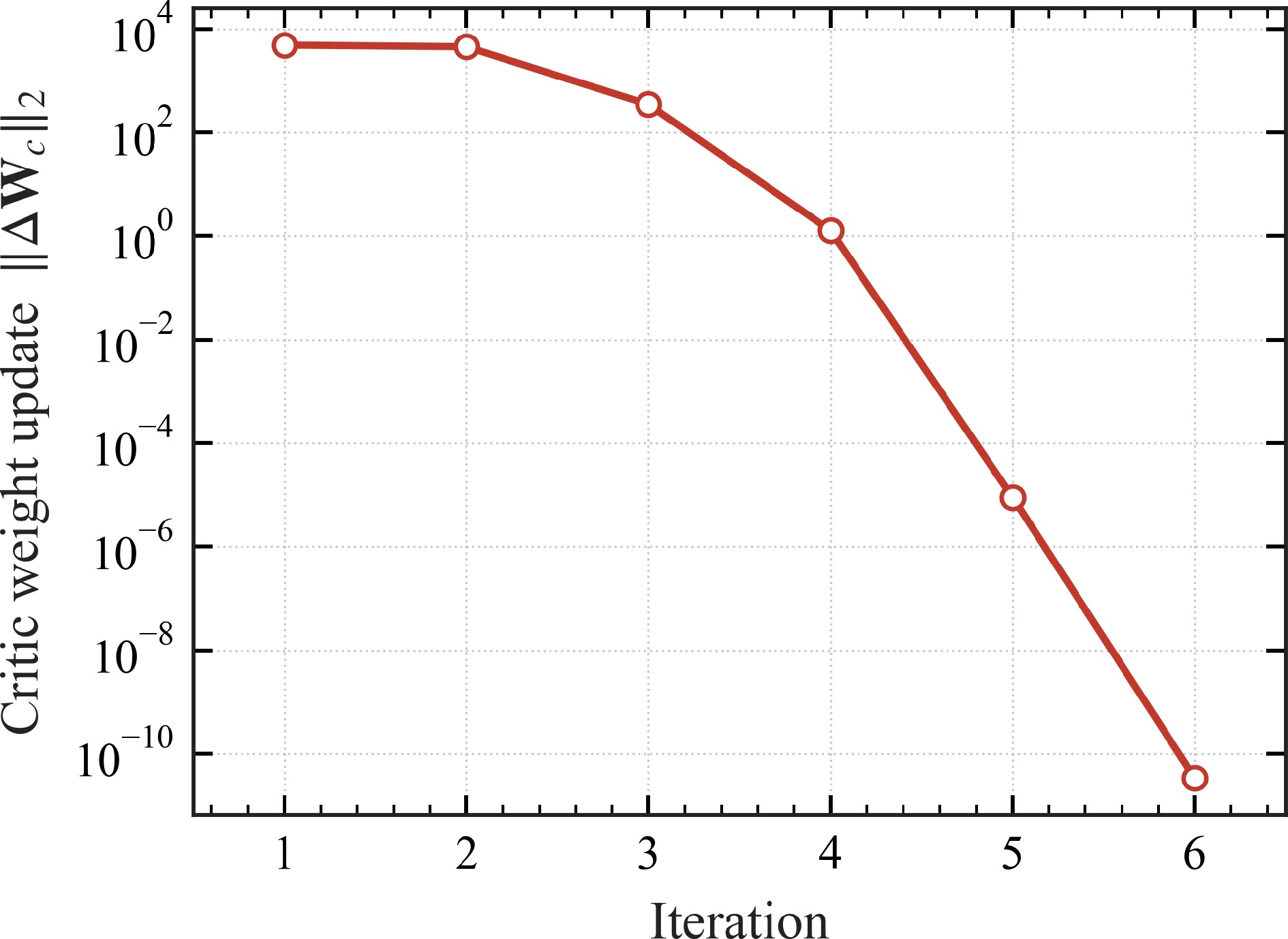
Figure 3.
Off-policy IRL convergence: per-iteration Critic-update norm $ \|\Delta{\boldsymbol{W}}_{c}\|_{2} $ vs policy-iteration index (logarithmic axis); the algorithm stops when this quantity falls below $ \varepsilon=10^{-6} $.
Figures 4 and 5 compare the learned policy against the CasADi optimum on the IRL-applied phase. Because the translational reference traces a slow circular path on the tilted contact plane (Table 1), the end-effector engages the surface, follows it through a varying-penetration arc, and disengages once the reference carries it clear of the plane; both the position error and the contact force therefore evolve over the IRL-applied phase rather than settling to a static operating point. The normal position error (Fig. 4) follows the CasADi reference throughout: a small transient at contact establishment is followed by a larger, geometry-driven excursion (peaking near 0.3 m) as the reference sweeps across the surface, and the IRL and CasADi traces remain indistinguishable through both features before returning to zero at disengagement. The normal contact force (Fig. 5) exhibits a brief overshoot (
$ \lesssim 0.5\,\mathrm{s} $ 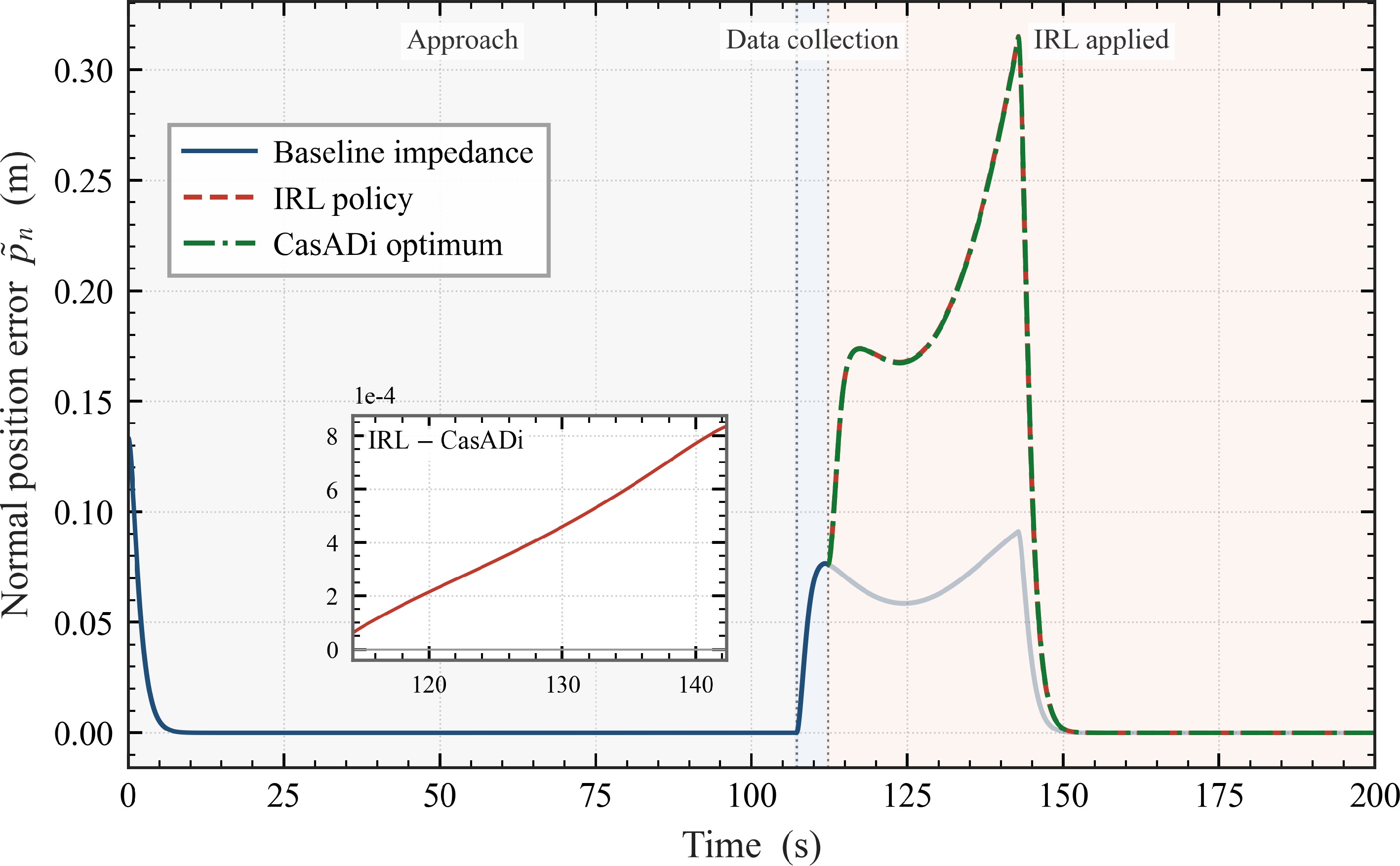
Figure 4.
Normal position error $ \tilde p_{n}(t) $: IRL policy vs CasADi optimum, with the noisy baseline shown across the full horizon for context. The inset shows the pointwise IRL$ - $CasADi difference over the regulated contact interval.
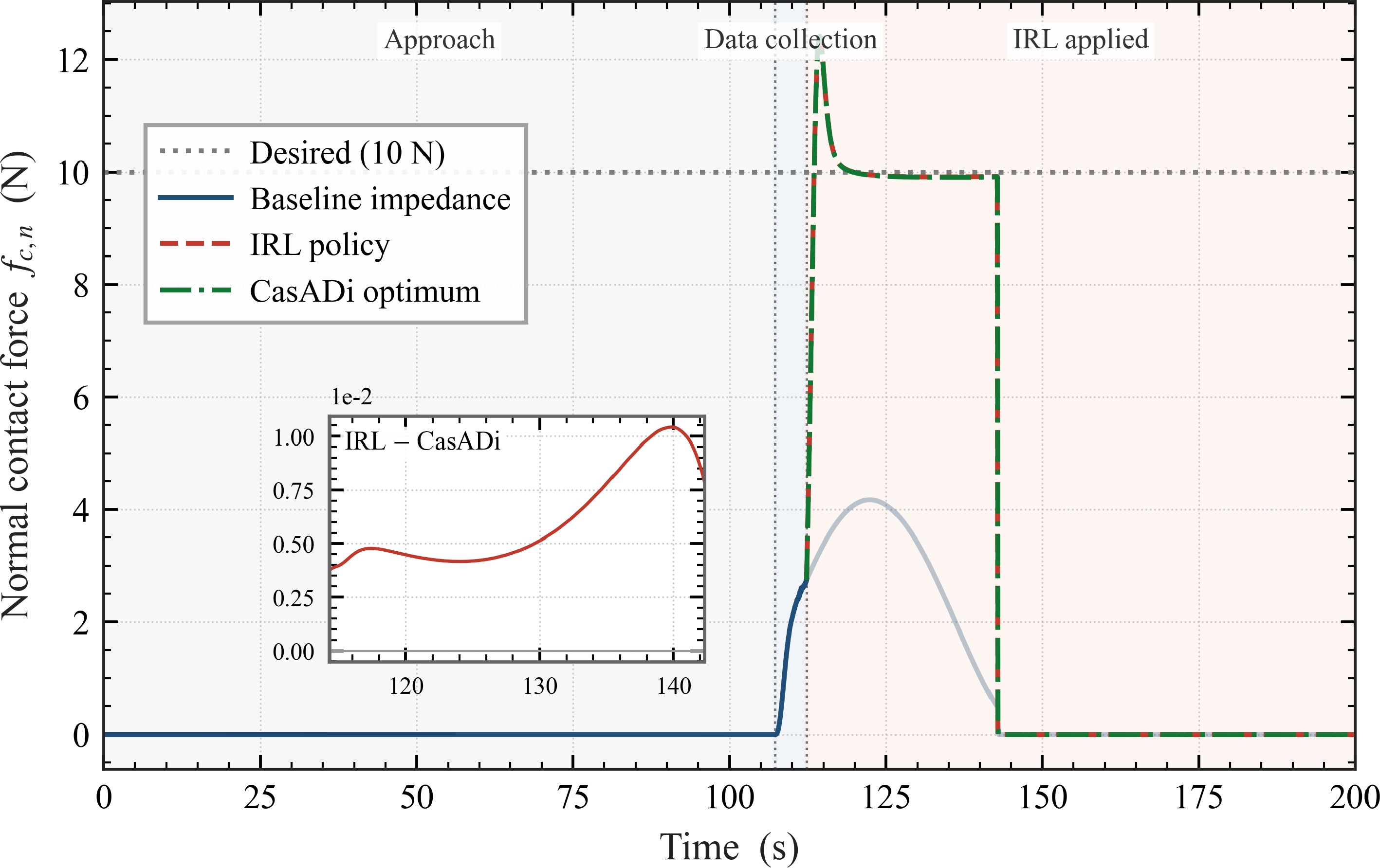
Figure 5.
Normal contact force $ f_{c,n}(t) $: IRL policy vs CasADi optimum, both regulating around the $ 10\,\mathrm{N} $ setpoint indicated by the dotted reference line. The inset shows the pointwise IRL$ - $CasADi difference over the regulated contact interval.
Robustness to different contact environments
-
The "Convergence and optimality" subsection fixed the deformation exponent at the default
$ n_{p}=1.5 $ $ n_{p} $ $ \{1.0,\,1.5,\,2.0\} $ $ n_{p}=1 $ $ n_{p}=1.5 $ $ n_{p}=2 $ $ k_{c} $ $ b_{c} $ $ f_{d,n} $ Were the contact the linear Kelvin–Voigt spring–damper
$ f_{c,n}=K_{\rm lin}\delta + c_{\rm lin}\dot\delta $ $ {\boldsymbol{z}}=[\dot\delta,\,\delta-\delta_{\rm eq}]^{\mathrm{T}} $ $ \delta_{\rm eq}=f_{d,n}/K_{\rm lin} $ $ n_{p} $ $ \bigl(\delta(t),\dot\delta(t),f_{c,n}(t)\bigr) $ $ f_{c,n}\approx K_{\rm id}\delta + c_{\rm id}\dot\delta $ $ \delta_{\rm eq}^{\rm id}=f_{d,n}/K_{\rm id} $ $ (K_{\rm id},c_{\rm id}) $ $ {\boldsymbol{K}}_{\rm fb} $ $ u_{n}=-{\boldsymbol{K}}_{\rm fb}\,{\boldsymbol{z}} $ $ {\boldsymbol{z}}=[\dot\delta,\delta-\delta_{\rm eq}^{\rm id}]^{\mathrm{T}} $ $ n_{p}=1 $ $ n_{p}>1 $ $ \to $ $ \to $ Figure 6 overlays the normal contact force traces for all three exponents on a single axis, with LC-LQR shown in orange dash-dot and the proposed IRL design in crimson dashed (lighter shade to darker shade as
$ n_{p} $ $ n_{p}=1 $ $ 10\,\mathrm{N} $ $ K_{\mathrm{id}}\approx k_{c} $ $ n_{p} $ $ 13\,\mathrm{N} $ $ n_{p}=1.5 $ $ 30\,\mathrm{N} $ $ n_{p}=2 $ $ 10\,\mathrm{N} $ $ \overline{|f_{c,n}-f_{d,n}|} $ $ \approx 0.13\,\mathrm{N} $ $ n_{p}=1 $ $ \approx 22\,\mathrm{N} $ $ n_{p}=2 $ $ \approx 1\,\mathrm{N} $ 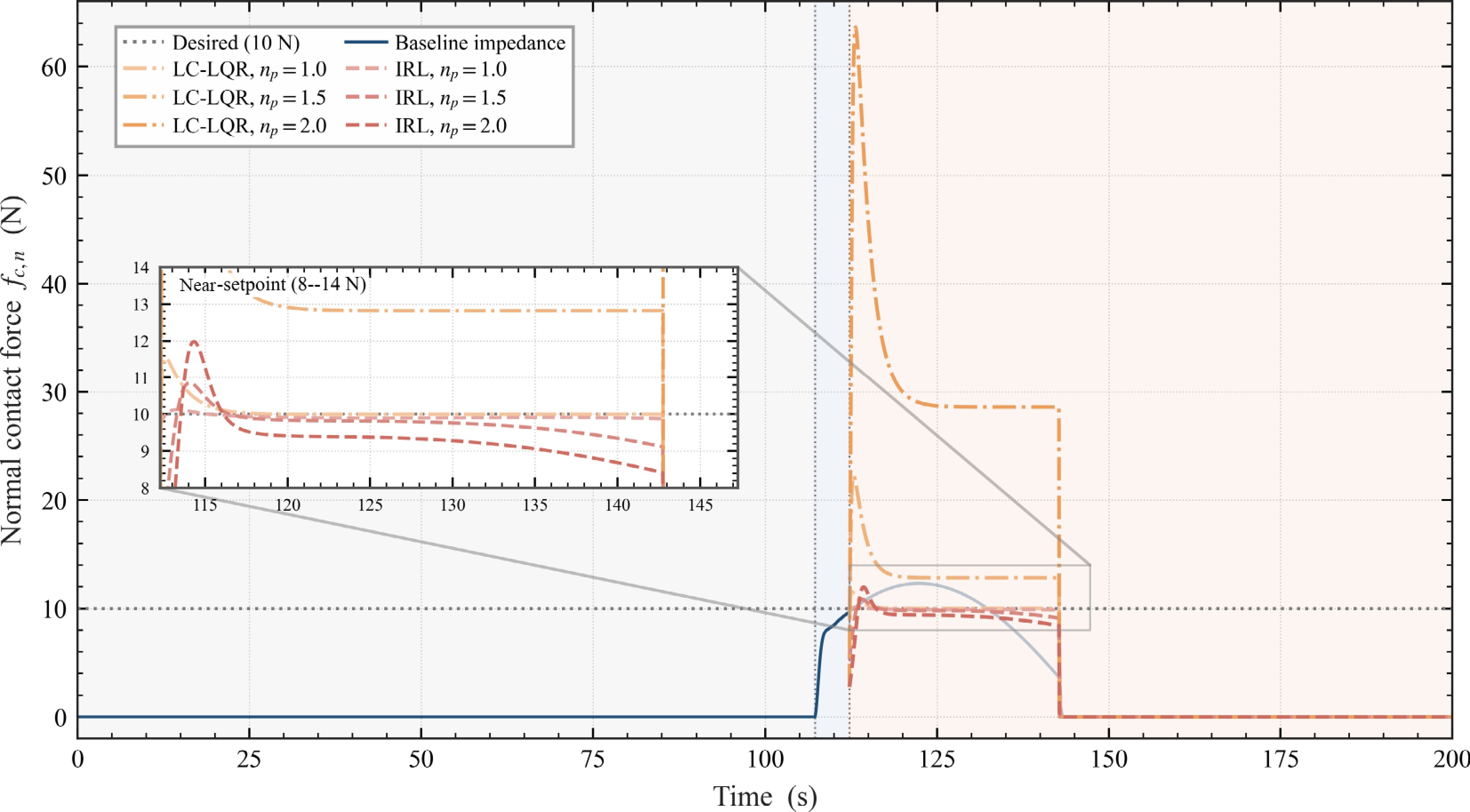
Figure 6.
Normal contact force $ f_{c,n}(t) $ for the three deformation exponents $ n_{p}\in\{1.0,1.5,2.0\} $, all overlaid on a single axis. Method is encoded by line style (LC-LQR dash-dot, IRL dashed), and $ n_{p} $ by colour shade (lighter $ \rightarrow $ darker as $ n_{p} $ grows). The shared noisy baseline is faded after the switch instant and the desired setpoint $ f_{d,n}=10\;\mathrm{N} $ is the dotted reference. Background shading marks the Approach/Data-collection/IRL-applied phases. The inset zooms the $ 8 $–$ 14\;\mathrm{N} $ band around the setpoint, exposing the near-setpoint tracking that the full vertical range compresses.
The influence of different weights
-
To probe the sensitivity of the learned policy to the cost weights
$ ({\boldsymbol{Q}},{\boldsymbol{R}}) $ $ {\boldsymbol{Q}} $ $ {\boldsymbol{R}} $ $ {\boldsymbol{Q}} $ $ {\boldsymbol{R}} $ $ f_{d,n} $ $ ({\boldsymbol{Q}},{\boldsymbol{R}}) $ Table 2. Cost-weight configurations for the sensitivity study.
Case $ {\boldsymbol{Q}} $ $ {\boldsymbol{R}} $ $ 1 $ (Aggressive) $ \mathrm{diag}(5\times 10^{4},\,5\times 10^{4},\,0) $ $ \mathrm{diag}(10^{-2},\,10^{-2}) $ $ 2 $ (Intermediate) $ \mathrm{diag}(5\times 10^{4},\,5\times 10^{4},\,0) $ $ \mathrm{diag}(10^{-1},\,10^{-1}) $ $ 3 $ (Compliant) $ \mathrm{diag}(5\times 10^{-5},\,5\times 10^{-5},\,0) $ $ \mathrm{diag}(1,\,1) $ Cases are ordered by decreasing $ {\boldsymbol{Q}}/{\boldsymbol{R}} $ ratio, i.e. from most aggressive to most compliant. Figures 7−9 compare the three configurations on the end-effector path in the contact plane, the normal position error
$ \tilde p_{n}(t) $ $ f_{c,n}(t) $ $ {\boldsymbol{Q}}/{\boldsymbol{R}} $ $ |\tilde p_{n}| $ $ \approx 0.12\,\mathrm{m} $ $ \approx 0.19\,\mathrm{m} $ $ \approx 0.20\,\mathrm{m} $ $ f_{c,n} $ $ 10\,\mathrm{N} $ $ \approx 9.7\,\mathrm{N} $ $ \approx 9.1\,\mathrm{N} $ $ \approx 5.5\,\mathrm{N} $ $ f_{d,n} $ $ \tilde p_{n} $ 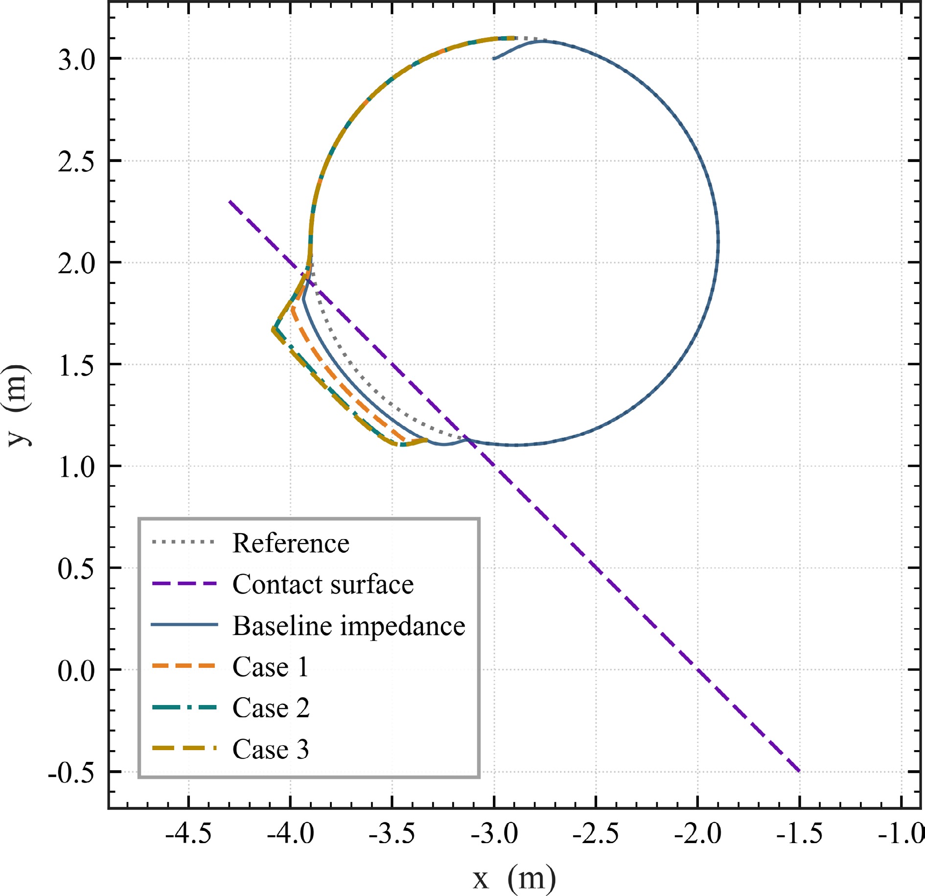
Figure 7.
End-effector path in the contact plane under the three weight configurations of Table 2, with the noisy baseline shown in light blue for reference.
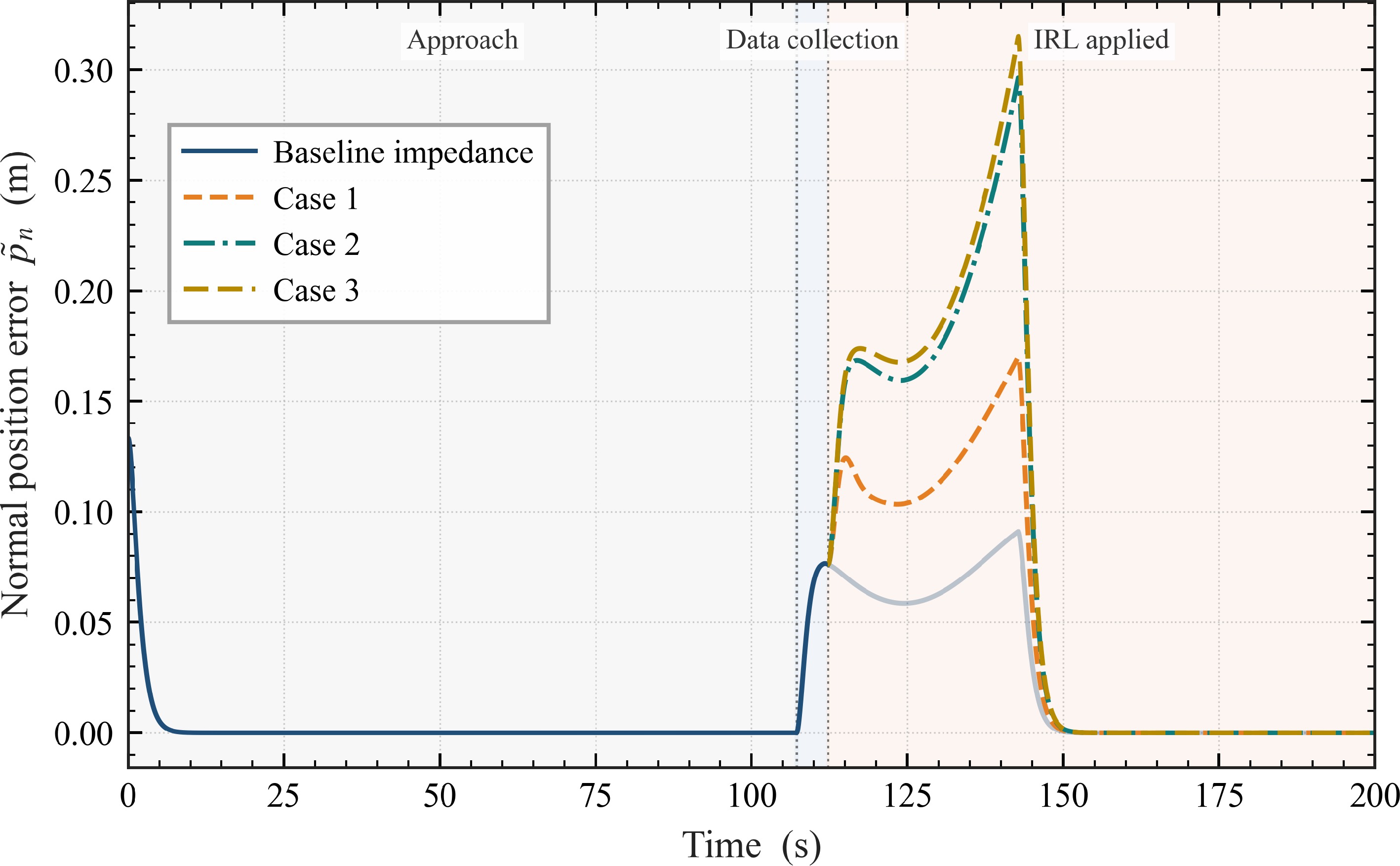
Figure 8.
Normal position error $ \tilde p_{n}(t) $ for the three weight configurations across the full simulation horizon. The shaded background marks the three pipeline phases.
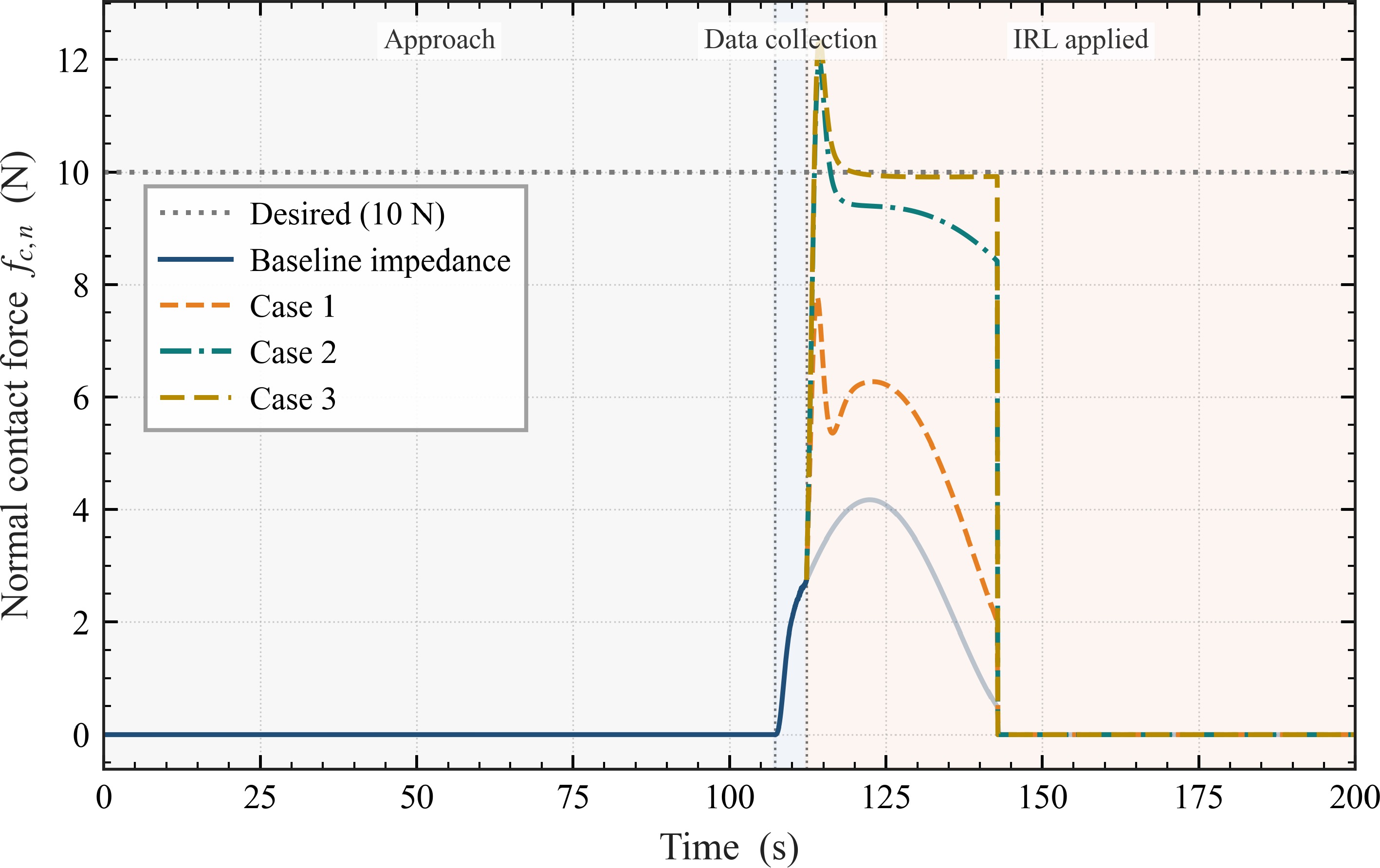
Figure 9.
Normal contact force $ f_{c,n}(t) $ for the three weight configurations across the full simulation horizon, regulated against the $ 10\,\mathrm{N} $ desired setpoint.
The end-effector path in Fig. 7 shows the same trade-off geometrically: the three IRL trajectories peel away from the (penetrated) reference circle by an amount that grows from Case 1 to Case 3, while remaining tangent to the contact surface for an increasingly long arc as the impedance is softened. Together, Figs 7–9 make the design implication explicit: the proposed cost (24) parameterizes a position-vs-force trade-off that the user navigates through
$ {\boldsymbol{Q}}/{\boldsymbol{R}} $ Discussion
-
The three studies together support the central claim of the paper: an off-policy IRL synthesis whose only contact information comes from sampled trajectories can deliver impedance-control performance that the analytical alternatives cannot. The "Convergence and optimality" subsection establishes that on the nominal HC contact the learned policy matches the numerically computed optimum, demonstrating that the polynomial-basis Critic and the integral Bellman equation are sufficient to recover the analytical solution from data. The "Robustness to different contact environments" subsection shows that as the contact moves away from the linear case, the proposed design retains tracking accuracy while LC-LQR— exact at
$ n_{p}=1 $ $ ({\boldsymbol{Q}},{\boldsymbol{R}}) $ The contrast in the "Robustness to different contact environments" subsection is not about LC-LQR being implemented poorly: the sample-based identification recovers the linear contact exactly at
$ n_{p}=1 $ $ K_{\rm id} $ $ \approx 100\,\mathrm{N/m} $ $ n_{p}=1 $ $ \approx 18\,\mathrm{N/m} $ $ n_{p}=2 $ $ \delta_{\rm eq}^{\rm id} $ $ f_{c,n}(\delta,\dot\delta) $ Two scope qualifications apply. First, the experiments restrict the contact-model variation to the deformation exponent of the HC family. The proposed design does not require this restriction—any smooth contact-force law fits in (12)—but the present paper does not test it on contact models outside the HC family (such as plastic or stick-slip contact). Second, the basis order
$ \deg({\boldsymbol{\sigma}})=4 $ $ (D_{n},K_{n}) $ -
This paper developed an off-policy integral reinforcement learning framework for optimal impedance control of aerial manipulators interacting with surfaces whose contact dynamics need not be modelled in advance. By projecting the Cartesian impedance equation onto the contact frame, taking the desired stiffness and damping along the dominant normal direction as virtual control inputs, and solving the resulting Hamilton–Jacobi–Bellman equation online with an Actor–Critic scheme, the design avoids committing to any specific contact-model parameterisation and avoids any pre-mission contact-parameter identification.
Numerical experiments on a Hunt–Crossley test contact verified the framework on three fronts. The learned policy matches an analytically computed reference optimum in force tracking and motion regulation, with the Critic weights converging within a small number of policy iterations under a polynomial basis. A sweep of the cost weights
$ ({\boldsymbol{Q}},{\boldsymbol{R}}) $ $ n_{p} $ $ (K_{\rm lin},c_{\rm lin}) $ $ n_{p} $ Future work will extend the framework to a fully coupled floating-base treatment and to tasks with time-varying contact geometry, and will pursue hardware-in-the-loop validation on a representative aerial-manipulator testbed.
This work was supported by the National Key R&D Program of China (2021YFC2202901, 2023YFC2206004, 2024YFC2207203), the National Natural Science Foundation of China (U25B2052), and the Heilongjiang Provincial Natural Science Foundation (YQ2024F010).
-
This study did not involve human participants, animals, or clinical data. Ethical approval was therefore not required.
-
The authors confirm their contributions to the paper as follows: conceptualization: Zhang Z, Tang X; methodology, software, visualization, and writing — original draft: Zhang Z; validation: Zhang Z, Xiao Y; project administration: Tang X; supervision, funding acquisition, and writing — review and editing: Tang X, Ye D; software, data curation: Xiao Y. All authors reviewed the results and approved the final version of the manuscript.
-
The datasets generated and analyzed during the current study, together with the source code reproducing all figures, are available from the corresponding author upon reasonable request.
-
The authors declare that there is no conflict of interest.
- Copyright: © 2026 by the author(s). Published by Maximum Academic Press, Fayetteville, GA. This article is an open access article distributed under Creative Commons Attribution License (CC BY 4.0), visit https://creativecommons.org/licenses/by/4.0/.
-
About this article
Cite this article
Zhang Z, Tang X, Xiao Y, Ye D. 2026. Contact-model-free optimal impedance control of aerial manipulators via off-policy integral reinforcement learning. International Journal of Micro Air Vehicles 18: e021 doi: 10.48130/mav-0026-0019 

Contact-model-free optimal impedance control of aerial manipulators via off-policy integral reinforcement learning
- Received: 29 May 2026
- Revised: 19 July 2026
- Accepted: 17 August 2026
- Published online: 30 October 2026
Abstract: This paper develops a contact-model-free adaptive impedance controller for aerial manipulators performing force-regulation tasks during operations on a planar surface. The proposed method requires no a priori parameterization of the contact dynamics; therefore, it can be applied to a wide range of practical scenarios. A contact-frame projection reduces the six-dimensional Cartesian impedance equation to a scalar normal-direction subproblem, while the friction-driven tangential channels are separately shown to be input-to-state stable. By taking the desired stiffness and damping along the normal direction as virtual control inputs and quantifying the interaction performance through a discounted value function, this subproblem is recast as a nonlinear optimal control problem with unknown dynamics. The associated Hamilton–Jacobi–Bellman (HJB) equation is solved online by an off-policy integral reinforcement learning (IRL) scheme operating on measured trajectories, and the optimal time-varying impedance gains are read directly from the Actor without post-hoc reconstruction. Finally, numerical experiments on a Hunt–Crossley test contact verify the effectiveness of the proposed controller. The results show that the proposed design retains tight force tracking across a family of nonlinear contacts, whereas a linear-contact LQR alternative degrades by orders of magnitude.