Watershed non-point source nitrogen apportionment: from qualitative to intelligence frameworks

Nitrogen (N) is a fundamental element of living organisms and plays a critical role in sustaining Earth’s ecosystems. In natural environments, N cycles among soils, water bodies, the atmosphere, and biota in the forms of ammonium, nitrate, and organic N, thereby sustaining the balance of the global N cycle^[1,2]. Since the Industrial Revolution, however, the extensive application of synthetic N fertilizers to support growing food demands has profoundly altered this cycle^[1]. Currently, over 100 Tg of fertilizer N are produced and applied annually worldwide, far exceeding inputs from natural biological N fixation^[3]. Although these inputs have greatly enhanced global food production, large amounts of N not taken up by crops are released into the environment, leading to a series of ecological and environmental problems, including acidification, loss of biodiversity, and water eutrophication^[4−6].

Agricultural non-point source (NPS) pollution is the major contributor to rising N loads in aquatic ecosystems worldwide^[7−9], from the Gulf of Mexico to Taihu Lake and the Baltic Sea^[10−12]. NPS is defined as dissolved or particulate N transported into water bodies via runoff and subsurface flow from multiple sources, including fertilizer application, livestock waste, rural domestic sewage, and atmospheric deposition. These N sources are characterized by dispersion, strong spatiotemporal variability, diverse hydrological pathways, and delayed hydrological responses^[12]. Moreover, mixing and biogeochemical transformation during N transport pathways further complicate the identification and quantification of N sources^[13−15]. Given these challenges, developing a reliable framework for watershed N source apportionment is crucial for understanding the mechanisms, identifying critical source areas, and informing effective NPS control strategies.

Although N exists in watersheds in various forms, including ammonium (NH₄⁺), nitrate (NO₃⁻), and dissolved organic N (DON), research specifically identifying the sources of NH₄⁺ and DON remains limited. For instance, recent approaches include using¹⁵N–NH₄⁺ to trace NH₄⁺ in marine, estuarine, and freshwater systems, and applying excitation–emission matrix and fluorescence spectroscopy to characterize the sources of DON in Poyang Lake^[16]. Nitrate, however, is the primary form of N loss from NPS pollution, because synthetic fertilizers and livestock manure are rapidly converted to NO₃⁻ through nitrification^[17]. In addition, NH₄⁺ tends to adsorb onto soil colloids and is resistant to migration, whereas the mineralization of DON requires a certain turnover time^[17]. Therefore, this study concentrates on the source apportionment of NO₃⁻ within the watershed to support the management of NPS pollution control.

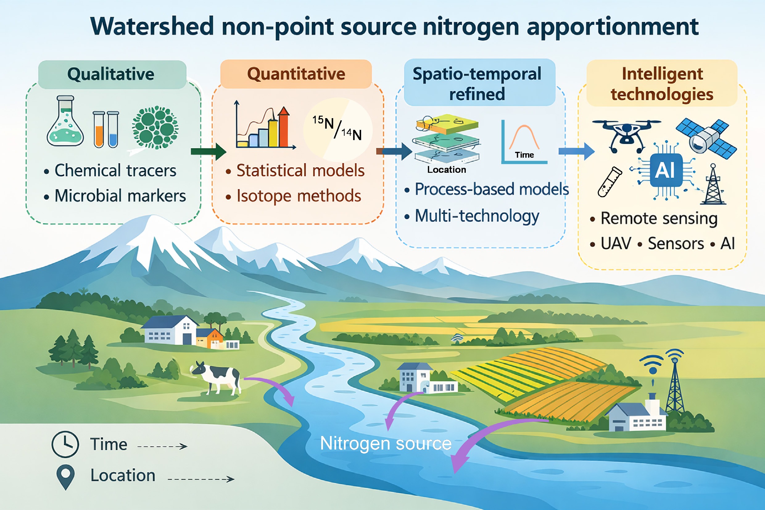
Advances have been achieved in N source apportionment (referring primarily to NO₃⁻; the same applies below) methods in recent years, supported by technologies spanning isotopic techniques, molecular biological tracers, process-based models, and remote sensing^[18−20]. Traditional watershed N source apportionment methods have shifted from qualitative to quantitative, spatiotemporally explicit, and intelligent frameworks, enabling the characterization of complex N dynamics in heterogeneous landscapes^[21,22]. However, no single method provides universal applicability. The various N source apportionment approaches differ in terms of their analytical precision, spatiotemporal applicability, and data requirements. Consequently, each method is optimally suited to specific environmental susceptibilities and management targets^[23−25]. These differences highlight the need for a more comprehensive understanding of the methodological foundations and characteristics of different approaches. To address these challenges, we synthesize the core principles, representative techniques, strengths, limitations, and recent advances of watershed N source apportionment, and, for the first time, classify these approaches into four major categories: (1) qualitative approaches, (2) quantitative approaches, (3) spatiotemporally refined approaches, and (4) intelligent technologies (Fig. 1 and Table 1). Finally, we identify critical gaps and priority research essential for developing precision and multiscale source apportionment systems that can effectively guide targeted watershed N management.

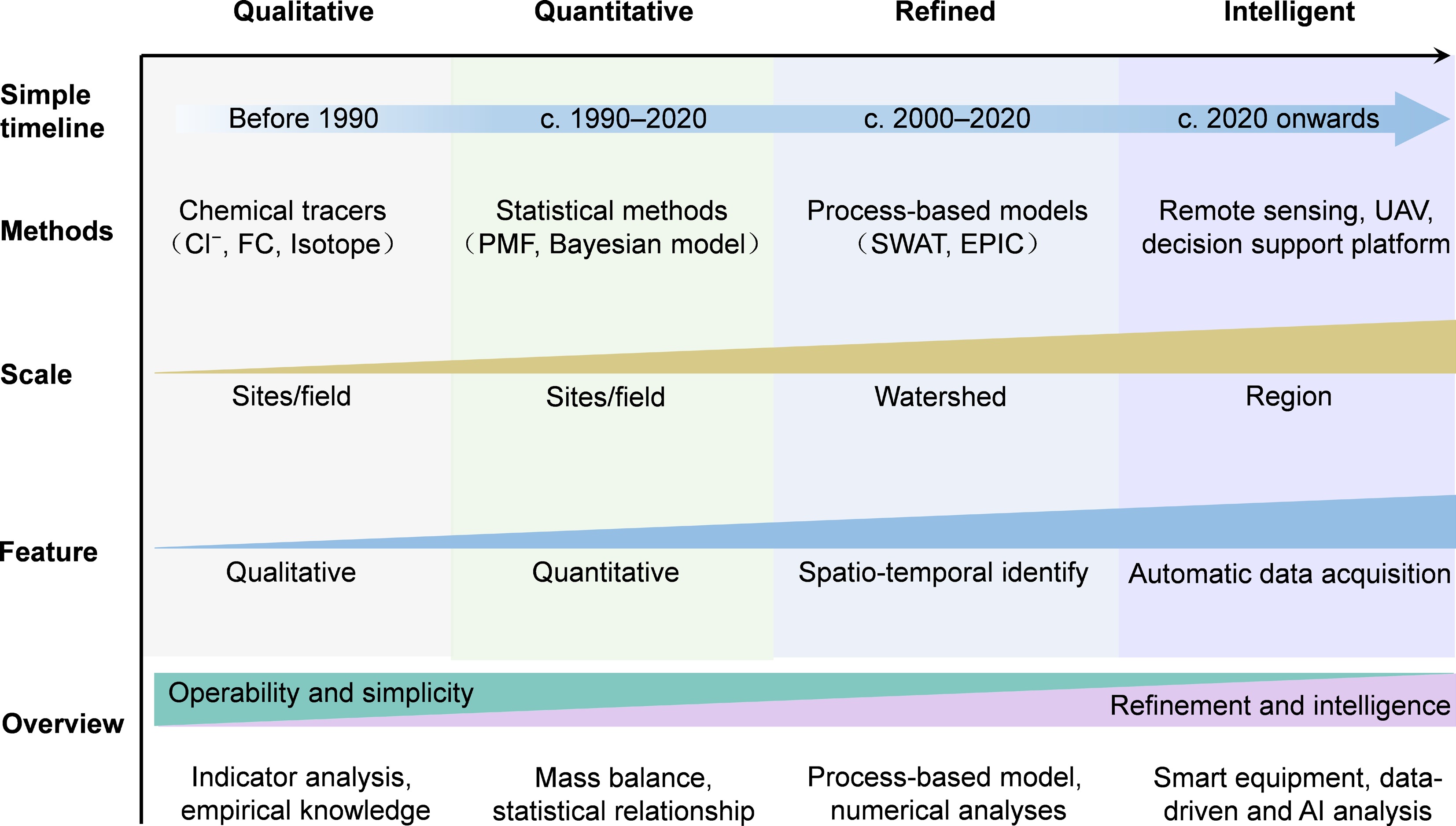
Figure 1. 

Classification and overview of methods for watershed nitrogen source apportionment. These methods are classified into four categories according to their objectives: qualitative approaches, quantitative approaches, spatiotemporally refined approaches, and intelligent technologies. Their corresponding methodological principles, applicability, and characteristics are described. FC, fecal coliform; PMF, positive matrix factorization; SWAT, soil and water assessment tool; EPIC, environmental policy integrated climate; UAV, unmanned aerial vehicle.

Inorganic ions such as Cl⁻, Ca²⁺, and B³⁺ have been widely used as rapid indicators for watershed N source apportionment since the 1990s^[34−36] (Fig. 2). Cl⁻ is particularly useful because of its conservative behavior in natural systems, where measured concentrations reliably indicate pollution sources' characteristics. Domestic sewage and livestock manure typically contain high Cl⁻ concentrations, whereas fertilizer-derived Cl⁻ concentrations are relatively low^[27]. Moreover, the NO₃⁻/Cl⁻ ratio can be further used to distinguish sewage inputs (higher ratios) from livestock waste (lower ratios), as sewage treatment typically reduces Cl⁻ concentrations^[26]. Other ionic tracers (e.g., Br⁻, I⁻, Na⁺, Ca²⁺, B³⁺, Sr²⁺) and isotopic ratios (δ¹¹B and⁸⁷Sr/⁸⁶Sr) can also serve as supplementary indicators for source identification^[37−39]. For example, leachate from waste disposal shows elevated Br⁻ due to organic waste degradation^[40,41], whereas groundwater δ¹¹B and ⁸⁷Sr/⁸⁶Sr vary among agricultural runoff, livestock effluent, and domestic wastewater^[42−44]. These indicators provide rapid qualitative identification of pollution sources; however, their reliability is often limited by environmental variability, as ion concentrations are affected by dilution, chemical reactions, and hydrological fluctuations. For example, heavy rainfall may rapidly leach fertilizer-derived NO₃⁻ while leaving Cl⁻ relatively stable, resulting in concentrations similar to those of sewage inputs, and denitrification further reduces NO₃⁻ and disrupts its relationship with Cl^−[45]. Such processes limit the reliability of these chemical tracers in complex or mixed-source watersheds.

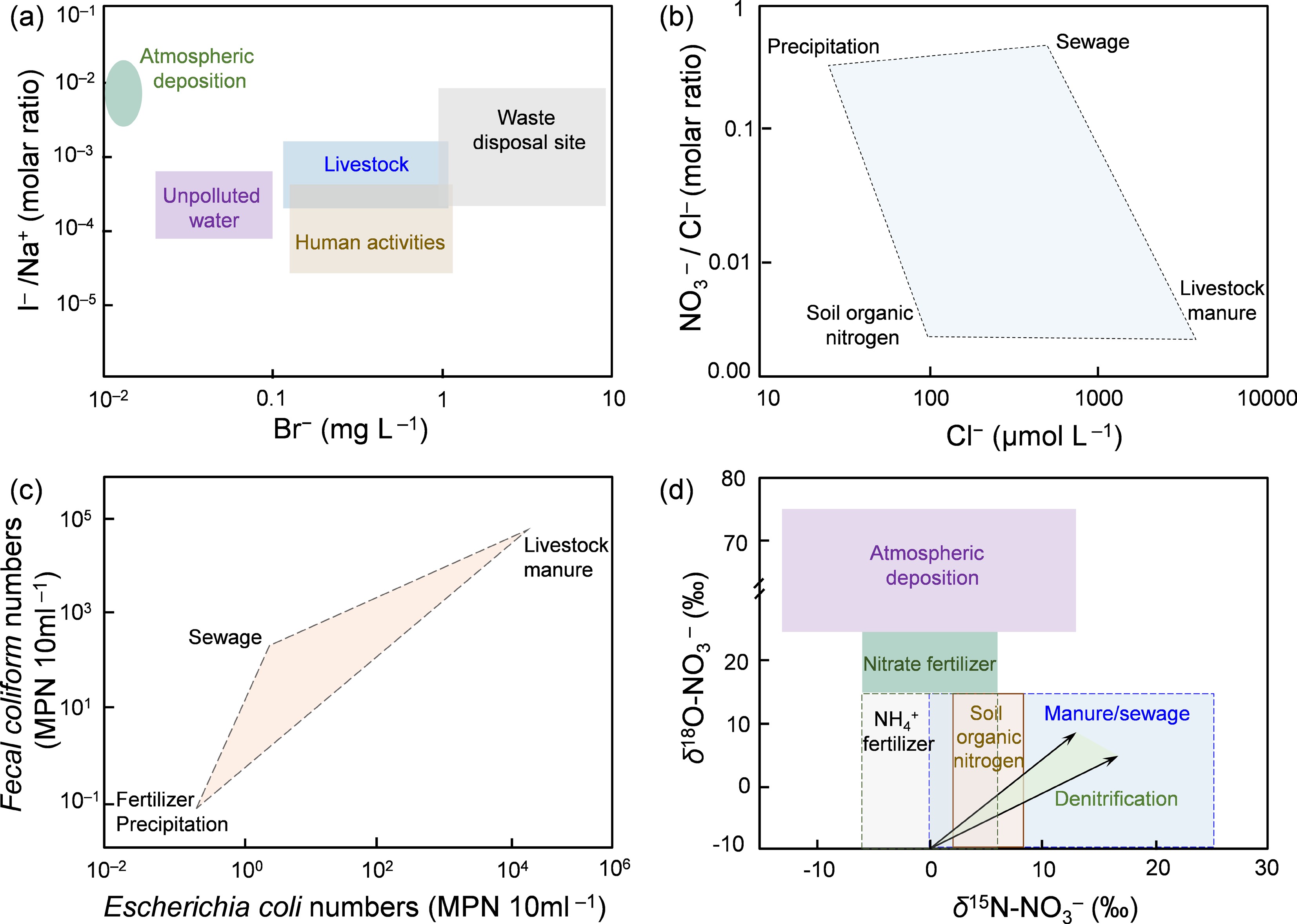
Figure 2. 

Representative qualitative methods for watershed nitrogen source apportionment. Different shades and positions represent the concentration and distribution characteristics of tracers from different sources.

Microbial indicators

Microbial markers are characterized by stronger specificity for identifying pollution sources than chemical element tracers^[46,47]. Animal feces and treated domestic wastewater contain much higher concentrations of Escherichia coli (EC) and fecal coliforms (FCs) than those in rainfall or fertilizers^[48,49] (Fig. 2c). Microbial markers stay effective despite the loss of diagnostic validity of NO₃⁻/Cl⁻ ratios caused by rainfall dilution or denitrification. For example, livestock-affected waters may exhibit NO₃⁻/Cl⁻ ratios similar to sewage during summer rainfall events, yet EC measurements still indicate the contribution of animal waste^[50]. Within complex N source landscapes, this source specificity compensates for the shortcomings of traditional source apportionment methods based on chemical element tracers. However, microbial survival and DNA integrity are highly sensitive to environmental factors. Temperature and pH strongly influence detection rates, and FC persists for several weeks at 4 °C but has a half-life of only 2–3 d in warm summer waters (> 25 °C)^[51,52]. These sensitivities underscore the necessity of accounting for ambient environmental factors during sampling when interpreting microbial marker data.

Use of δ¹⁵N and δ¹⁸O isotopes in nitrate for qualitative identification

Unlike easily degradable microbial markers, δ¹⁵N and δ¹⁸O isotopes in NO₃⁻ are relatively stable in aquatic systems and are less affected by environmental factors^[53,54]. As N is transported in watersheds, the element undergoes biogeochemical processes such as mineralization, nitrification, denitrification, and ammonia volatilization, leading to isotope fractionation effects. These effects result in distinct δ¹⁵N and δ¹⁸O signatures across varying sources, which are extensively applied to identify N pollution sources^[55,56] (Fig. 2d). For example, NO₃⁻ from feces and sewage typically shows elevated δ¹⁵N (+10‰ to +15‰) caused by preferential consumption of light isotopes during organic matter decomposition and denitrification^[57], whereas soil δ¹⁵N–NO₃⁻ (+3‰ to +8‰) is close to that of atmospheric NO₃⁻ (−3‰ to +7‰)^[58]. Atmospheric deposition generally exhibits higher δ¹⁸O–NO₃⁻ (+25‰ to +75‰), whereas fertilizer-derived NO₃⁻ has lower δ¹⁸O (+15‰ to +25‰)^[59]. Establishing a source-specific δ¹⁵N–NO₃⁻ and δ¹⁸O–NO₃⁻ database would enable the qualitative identification of NO₃⁻ sources. Nevertheless, δ-values from different sources may overlap, such as δ¹⁵N–NO₃⁻ from mineralized soil and fertilizer N, and in-stream N cycling may further reshape isotopic signatures^[26,30,60]. Therefore, combining chemical indicators, microbial markers, and isotopic techniques alongside watershed hydrology and environmental conditions would enhance the reliability of watershed N pollution source identification.

Multivariate statistical methods have been applied to quantify contributions from different non-point pollution sources, such as absolute principal component–multiple linear regression (APCS-MLR) and positive matrix factorization (PMF) models^[61,62]. These methods typically establish a mass balance between pollutant concentrations in samples and potential sources via mathematical solutions to estimate the sources' contributions. For example, PMF was used to identify feces and sewage as the dominant NO₃⁻ sources in Poyang Lake groundwater, contributing over 50% of the N load^[63]. The key advantage of these methods is that they do not require prior knowledge of the sources' characteristics (e.g., the specific categories of local pollution sources); however, source identification relies heavily on the researcher's judgment and can be influenced by data quality and the lack of a description of the processes. Similarly, the export coefficient method, based on pollutant runoff and retention ratios, can also quantify watersheds' non-point source contributions^[64−66]. This approach is simple and easy to implement with few data requirements, but it fails to account for pollutants' transport and transformation, leading to substantial uncertainty in source apportionment.

Stable nitrate isotopes for quantitative source apportionment

Isotopic signal can be used not only to qualitatively identify the sources of N pollutants but also to quantitatively apportion them when combined with an end-member mass balance framework. Unlike multivariate statistical models that operate without prior information on pollutant sources, isotope-based approaches with δ¹⁵N–NO₃⁻ and δ¹⁸O–NO₃⁻ are considered to be more robust because the isotopic signatures of potential sources are known in advance^[28,29,67]. The general workflow involves collecting isotope signatures from representative sources such as fertilizers, soils, livestock manure, domestic sewage, and atmospheric deposition, followed by establishing a mathematical relationship between these end-members and the isotopic composition measured in polluted water bodies. SIAR and MixSIAR models with a Bayesian framework are widely used to estimate source contributions as follows:

where, $ {X}_{ij} $ represents the value of isotope $ j $ in sample $ i $ ($ i $=1, 2, 3,…, N; $ j $=1, 2, 3,…, J), $ {S}_{jk} $ is the value of isotope $ j $ in source $ k $ ($ k $=1, 2, 3,…, K), $ {\mu }_{jk} $ is the mean value, $ \omega _{jk}^{2} $ is the variance of the normal distribution, and $ {C}_{jk} $ is the fractionation factor for isotope $ j $ in source $ k $ with a mean $ {\gamma }_{jk} $ and the variance $ \tau _{jk}^{2} $, and $ {p}_{k} $ is the contribution of source $ k $ estimated by the model. The residual term $ {\varepsilon }_{ij} $ represents unexplained variability with a mean of zero and variance of $ \sigma _{j}^{2} $.

The Bayesian isotope model offers the advantage of quantifying the uncertainty range of source contributions and the isotopic fractionation associated with in-stream denitrification. Denitrification is widespread in river systems and shifts δ¹⁵N by approximately −40‰ to −5‰ and δ¹⁸O by approximately −16‰ to −4‰; neglecting this process increases the uncertainty in nitrate source apportionment^[56,68,69]. Within Bayesian frameworks, the fractionation coefficient can be estimated using the Rayleigh formulation, which assumes a linear relationship between the residual nitrate and the isotopic value:

where, $ {\delta }_{Rt} $ represents the isotopic value at time $ t $, $ {\delta }_{R0} $ is the initial isotopic value in nitrate, $ f $ is the proportion of residual nitrate in the water body, and $ \varepsilon $ is the fractionation coefficient.

Although isotopic Bayesian models are widely applied for quantitative nitrate source apportionment, several limitations remain in practice. First, overlaps in isotopic signatures among different sources compromise source discrimination, particularly between livestock manure and domestic wastewater^[55]. Source signatures also vary across regions and seasons. For example, a survey of 28 vegetable planting greenhouses in Zhejiang Province showed that soils to which organic fertilizer had been applied had significantly higher δ¹⁵N values (mean = 7.97‰) than those with chemical fertilizers (mean = 5.13‰)^[70]. In addition, the selection of source categories, specification of the models' parameters, and the definition of prior information also influence the accuracy and uncertainty of Bayesian models' results^[57,71].

Although statistical methods quantify the total contribution of N loads, these approaches provide limited information on the spatial (e.g., location and transport pathways) and temporal (from hours to months and decades) origins of pollution within the watershed (Fig. 3). Process-based hydrological models simulate the generation, transport, and transformation of N from source to sink, thereby providing explicit spatial and temporal patterns of pollutant loss^[72]. These models integrate climate variability, land-use configuration, and fertilizer intensity to provide scenario assessments and policy evaluations for watershed N source apportionment, such as the soil and water assessment tool (SWAT), AGNPS, HSPF, and WPLT^[73−76]. For instance, SWAT combined with multivariate statistics successfully identified critical source areas in the Choctawhatchee watershed, where 28% of the land area accounted for 47% of total N export^[77]. HSPF was applied to quantify the spatiotemporal distribution of N loading across sub-basins in the Rappahannock watershed^[78]. Using historical human activity and meteorological data, long-term and daily nitrate exports (1980–2010) at hydrologic response units were simulated with SWAT in an intensive agricultural catchment of Southwestern France^[79]. Despite these advantages, process-based models require extensive model parameters, which are often limited in data-scarce regions^[25,80].

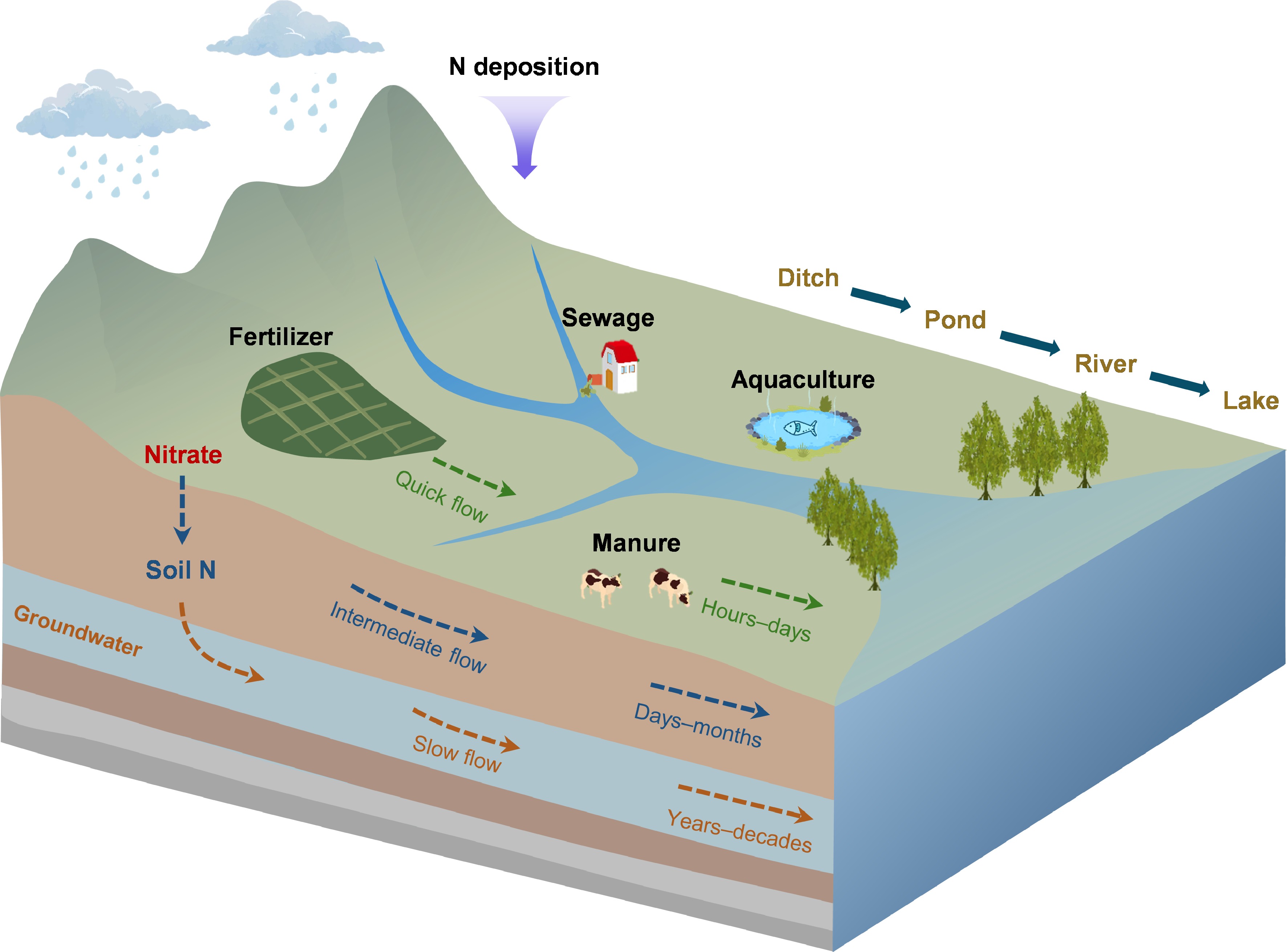
Figure 3. 

Processes and spatiotemporal characteristics of nitrogen transport in watersheds. Watersheds' non-point sources of nitrogen typically include fertilizer, livestock waste, rural domestic sewage, atmospheric deposition, and aquaculture. These pollutants are transported into water bodies through the surface, vadose zone, and groundwater as quick, intermediate, and slow flow, with travel times spanning from days to months and decades.

To reduce the complexity and data requirements of fully process-based models, semiempirical and process models that integrate empirical relationships and mechanistic processes have been developed to identify watershed N sources. Representative models such as SPARROW, IMAGE-GNM, NutriShed, and DPSs balance data requirements and detailed descriptions of the processes, thereby maintaining accuracy at large-scale estimates^[72,81−83]. For instance, the NutriShed model simulates pollutant transport and removal along flow paths and identifies N source contributions at a grid-level resolution^[82]. With the NutriShed model at a 30 m × 30 m resolution, 71% of the N runoff from croplands was estimated to be removed in a typical rice watershed in southern China^[82]. Overall, semiempirical and process models provide a practical compromise between mechanistic detail and data availability, with acceptable accuracy and broad applicability (Table 2).

Numerical analysis methods

In addition to non-point source pollution models, approaches that rely on hydrological analyses and numerical simulations also provide refined spatiotemporal source apportionment. For example, by combining hydrological partitioning with end-member mixing analysis, the contributions of surface flow, subsurface flow, and baseflow to total N and nitrate under different land-use types were distinguished in the Qinhuai River Basin^[84]. On the basis of δ¹⁵N–NO₃⁻ and δ¹⁸O–NO₃⁻ with N transformation modeling, the rates of nitrate transport, nitrification, and denitrification in surface–subsurface systems were identified in the Cane Run karst watershed in Kentucky^[85,86]. Furthermore, by incorporating the connectivity index of surface–vadose zone–groundwater and the SIAR model, researchers identified the N source types, spatial location, and transport pathways^[87]. Moreover, these isotopic data and numerical simulation approaches can further be combined with process-based models to quantify the dynamics of N sources, transformations, land-use contributions, and the drivers of watershed N transport^[88,89].

With the rapid development of intelligent equipment for watershed management, N source apportionment is shifting from low-frequency, field sampling toward data-rich, mechanism-informed, and intelligent online systems (Fig. 4). To distinguish it from spatiotemporally refined N source apportionment, we define intelligent methods as necessarily including equipment such as satellite-based remote sensing, unmanned aerial vehicles (UAVs), and in situ sensor networks to automatically collect high-frequency, real-time, long-term, or large-scale data. These devices not only facilitate the collection of such data but also integrate environmental data with numerical algorithms to support N source apportionment and watershed management.

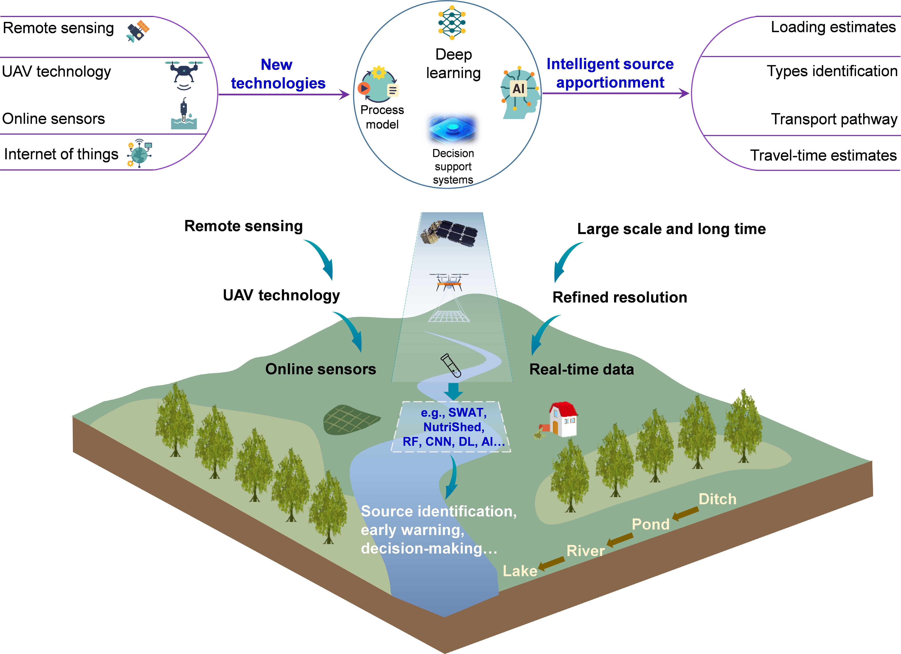
Figure 4. 

Intelligent technology and prospects of watershed nitrogen source apportionment. The intelligent source apportionment system acquires data via remote sensing, UAV, and sensor technologies, integrating process-based models with AI-driven data processing to characterize the dynamics of pollutant transport. This system has the advantages of large-scale monitoring and high-resolution spatiotemporal analysis, as well as providing targeted decision-making support for watershed management.

Intelligent technologies for large-scale N source apportionment

Intelligent technologies provide a unique advantage for N source apportionment at large spatial scales by enabling spatially extensive observations across heterogeneous watersheds. Traditional field-site monitoring is often insufficient to represent complex landscape configurations and hydrological connectivity for watersheds, leading to large uncertainties in source attribution at regional or basin scales. In contrast, satellite-based remote sensing and UAV-based imaging offer large-scale spatially explicit information that bridges water quality patterns with upstream landscape characteristics and management practices. For example, the DPeRS model integrates remote-sensing imagery and meteorological data to dynamically predict the contribution of agricultural activities to water pollution in large-scale watersheds^[32]. Additionally, machine learning algorithms such as Random Forest have been coupled with UAV imagery to accurately delineate subsurface agricultural drainage networks, providing critical data for pathway-specific source attribution^[90,91]. These technologies offer advantages in large-scale monitoring that can not be achieved by field-site monitoring.

Intelligent technologies for refined resolution N source apportionment

Compared with manual monitoring, another key advantage of intelligent monitoring technologies is their capacity to generate high-frequency and long-term observations. Such data are critical for elucidating N transformation and transport processes, as conventional weekly or monthly sampling fails to capture rapid concentration dynamics and often misses hydrologically driven key events. In contrast, automated data acquisition at an hourly or subhourly resolution provides a more detailed interpretation of pollutants' transport processes. Through the use of high-frequency sampling and isotope techniques, the distinct contributions of surface, subsurface, and groundwater to river water's quality during spring and summer were identified^[92]. The relative contribution of different hydrological components to riverine N loading during storm events was distinguished, based on high-frequency sampling of isotopic data^[93]. Sentinel-2 images were used to map the detailed spatial patterns of water quality along seven major rivers in Zhejiang Province from downstream to upstream, allowing the identification of long-term transport pathways^[33]. Moreover, the application of high-frequency monitoring technologies to elucidate the processes of water quality pollution during extreme precipitation events is crucial for mitigating the challenges of climate change.

Integrated platforms for intelligent N source apportionment

With the accumulation of multisource datasets and the development of source apportionment methods, intelligent source apportionment is increasingly implemented through integrated operational platforms. These systems typically include modules for data acquisition, analysis and processing, visualization of the results, and decision support. International projects such as the SmartWaters system in Europe and the NGWOS, BASINS, and WMOST platforms in the United States demonstrate the potential of such integrated systems to provide timely evaluations of pollution sources, forecast high-risk regions, and support cost-effective watershed management strategies^[94]. Though SmartWaters excels in high-frequency sensor data integration for European catchments, BASINS primarily focuses on providing comprehensive geographic information system (GIS)-based frameworks for long-term regulatory assessment across diverse North American landscapes. However, a common limitation across these systems is the inadequate mechanistic representation in highly complex watershed conditions. In China, rapid progress has been made in constructing national monitoring networks and digital river basin simulation systems such as the Yangtze and Yellow River Simulators. Nevertheless, important challenges remain regarding (1) insufficient integration across departmental data systems and the construction of standard databases; (2) inadequate mechanistic representation under complex watershed and hydrological conditions; and (3) weak connections among system modules for field monitoring, source identification, early warning, and decision-making.

To address these limitations of current source apportionment technologies, several key research focuses are expected to be advanced in future studies (Table 3). First, heterogeneous datasets from remote sensing, UAV, and in situ sensors vary in their spatiotemporal resolution and accuracy, limiting the feasibility of their combined application. Developing integrated space–air–ground monitoring platforms, together with standardized databases and automated preprocessing workflows, is expected to provide a robust foundation for model inputs. Second, more refined representations of pollutant transport, especially under complex watershed conditions and extreme events, are needed to improve models' generality and spatiotemporal accuracy. The understanding of N's source–flow–sink transport would benefit from the development of a unified framework that couples statistical models, process-based models, and isotope tracing. Finally, decision support systems should be further integrated with artificial intelligence technologies and large language models to enhance their accessibility and operational utility. For example, by integrating UAVs and deep learning, GeoAI can monitor compost heaps' volume and footprint to assess non-point source pollution^[90]. By integrating scenario simulation and cost–benefit analyses, such systems can support adaptive watershed management while providing interactive, user-friendly interfaces that lower application barriers and facilitate the implementation of intelligent watershed management.