-
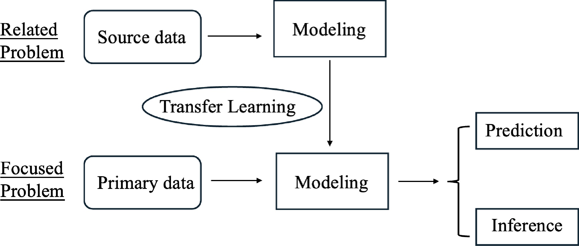
Figure 1.
An illustration of transfer learning. The goal is to build predictive models and conduct inference in the primary data for the focused problem. The modeling parameters learned from the source data of a related problem are transferred to the modeling process in the primary problem.
-
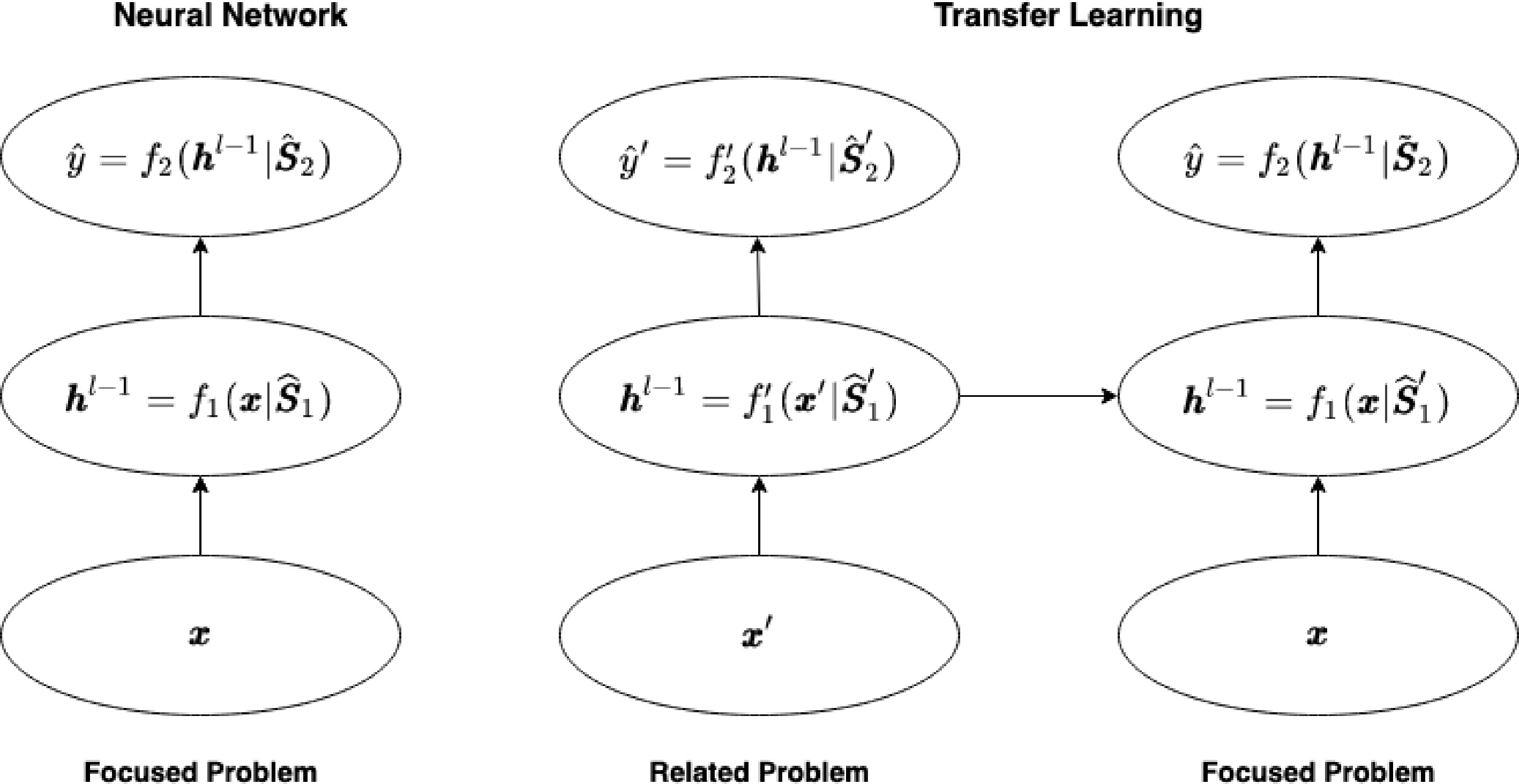
Figure 2.
Transfer learning in deep neural networks. The left panel shows the application of neural networks in the focused problem while the right panel displays the proposed transfer learning method based on training the neural networks in the related problem. Here
$ \hat{{\boldsymbol{S}}}_1' $ $ \tilde{\boldsymbol{S}}_2 $ $ \hat{{\boldsymbol{S}}}_1' $ -
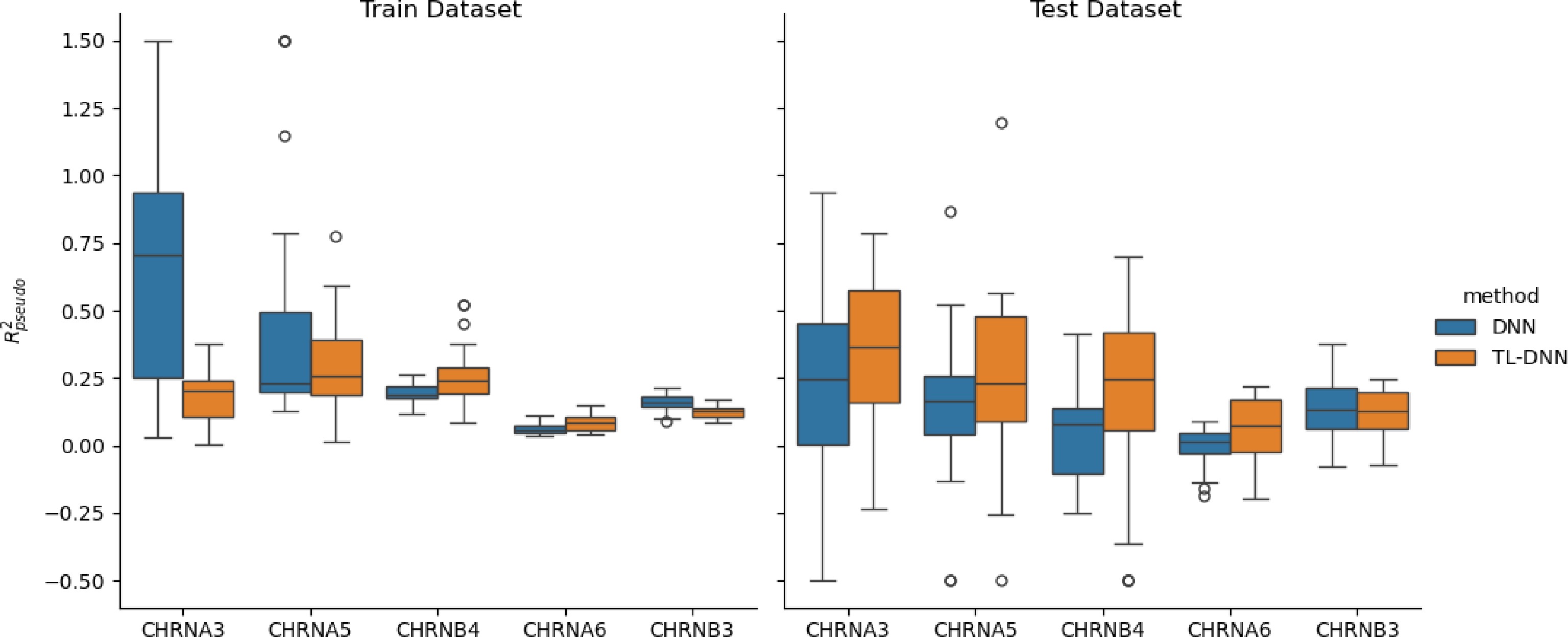
Figure 3.
Prediction comparison regarding relative efficiency in the SAGE data set between the transfer learning (TL-DNN) from UK Biobank and the direct application of DNN without transfer learning.
-
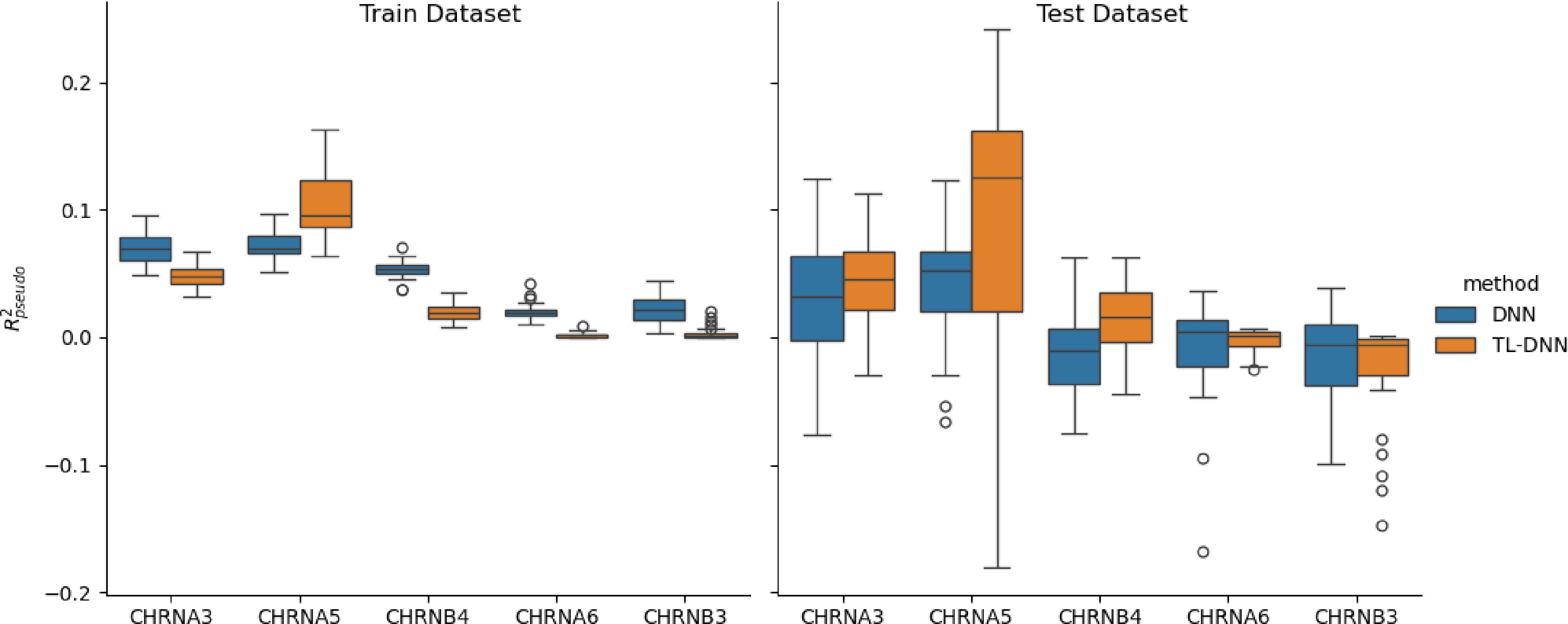
Figure 4.
Prediction comparison regarding relative efficiency in the SAGE data set between the transfer learning (TL-DNN) from UK Biobank and the direct application of DNN without transfer learning.
-
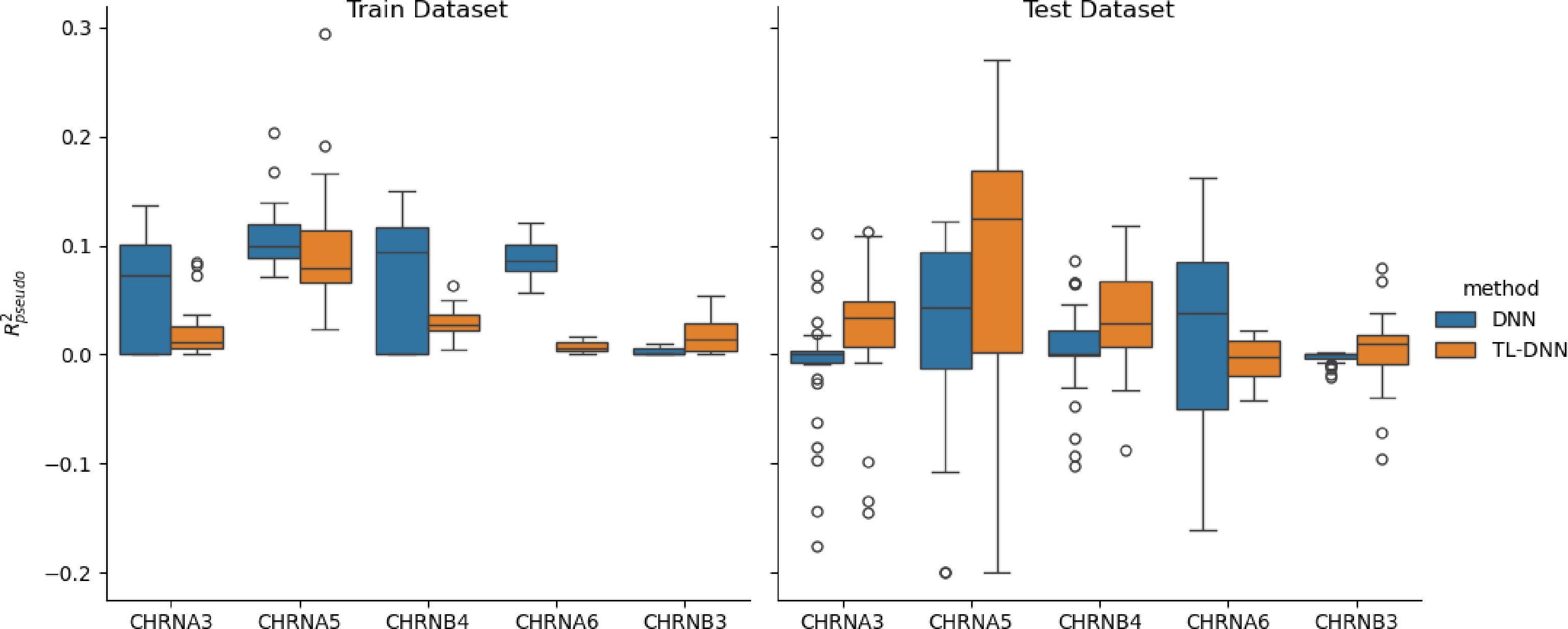
Figure 5.
Prediction comparison regarding relative efficiency in the UKB black population between the transfer learning (TL-DNN) from the white British population and the direct application of DNN without transfer learning.
-
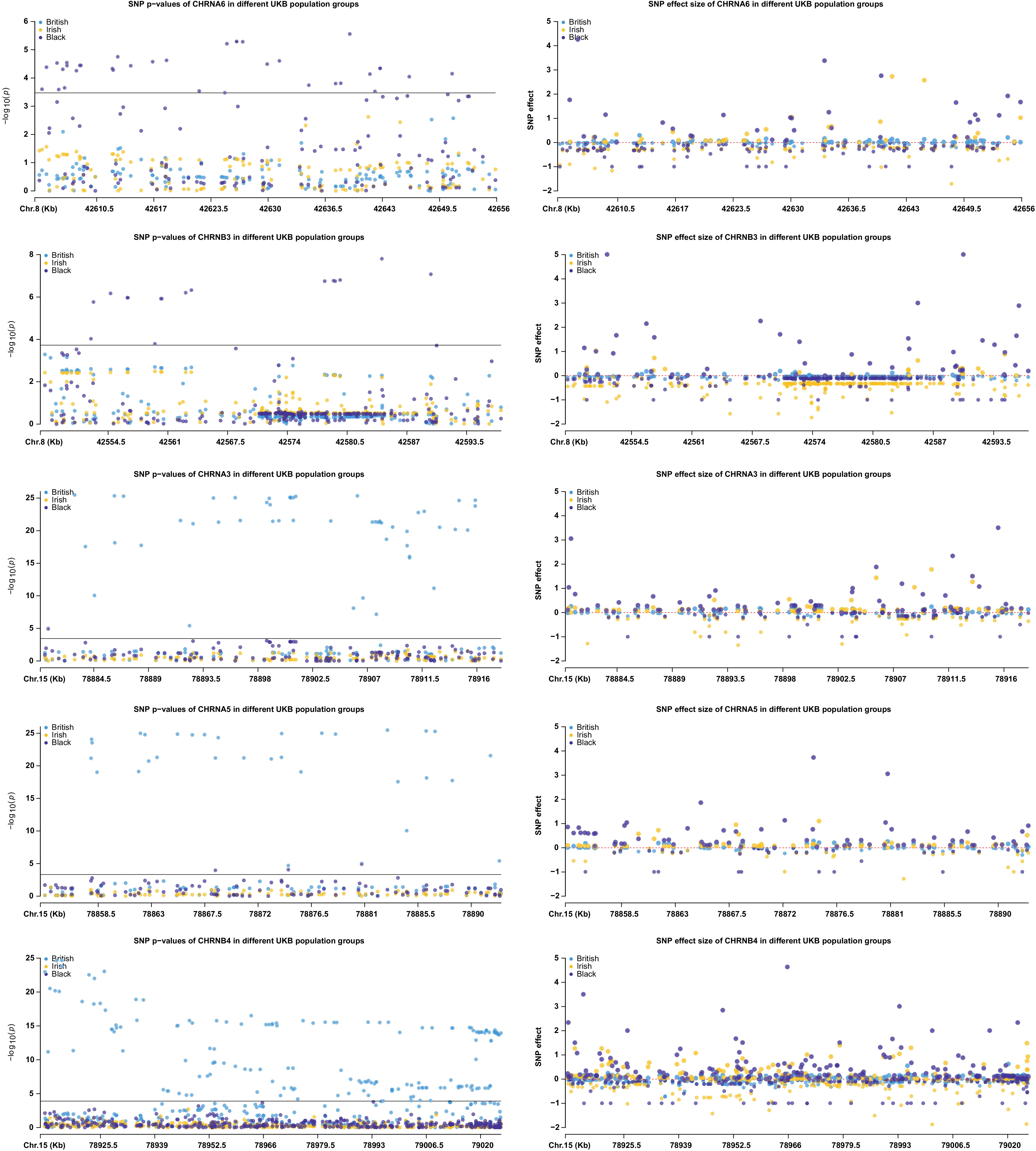
Figure 6.
Illustration of genetic heterogeneity among the ethnic UKB population groups regarding individual SNP p-values and affect sizes of the five genes in populations white British, white Irish, and black.
-
Permutation-based test using transfer learning with K-fold cross-validation Input: Genetic variants of a gene x, Phenotype y, a set of candidate smooth Group Lasso regularization parameters λSGL. Output: Empirical p-value of the gene Step 1: Construct a TL-DNN model f(x) with 2 hidden layers. Step 2: For k $ \leftarrow $ 1: Split (xtrain, ytrain), (xtest, ytest). For each λi in λ do a: Input (xtrain, ytrain) and train f(xtrain, ytrain;λi) with smooth Group Lasso regularization parameter λi, output $ \hat{f} $ b: Evaluate Mean Square Error on (xtrain, ytrain) , $ MSE(y_{test},\hat{f}(x_{test};\lambda_i)) $ end. 2: Choose λopt with the lowest MSE, output $ \hat y_{test} = \hat{f}(x_{test};\lambda_{opt}) $ $ MSE(y_{test}, \hat{f}(x_{test};\lambda_{opt})) $ 3: Permute $ x_{test} $ $ x_{test}' $ $ \hat y_{test}' = \hat{f}(x_{test}';\lambda_{opt}) $ $ MSE(y_{test}, \hat y'_{test}) $ $ l = MSE(y_{test}, \hat y_{test})-MSE(y_{test}, \hat y_{test}') $ 4: Repeat 3 for B times, obtain $ l_1,...,l_B $ $ \Delta_k = \frac{1}{B}\sum_{b = 1}^{B}l_b $ $ \hat{\sigma}_k^2 = var(l_1,...,l_B) $ end. Step 3: Calculate statistic $ \Delta = \frac{1}{K}\sum\Delta_k $ $ N(0, \sigma^2 = \frac{1}{K} \sum_{1}^{K} \sigma_k^2) $ end. Table 1.
Algorithm for the permutation-based association test using transfer learning.
-
Gene $ \Delta $ $ \hat\sigma $ p-value CHRNA3 −1.33e−3 1.10e−4 0 CHRNA5 −1.13e−3 1.01e−4 0 CHRNA6 −8.24e−5 3.19e−5 4.88e−3 CHRNB3 −1.20e−4 4.13e−5 2.19e−3 CHRNB4 −1.4e−3 1.11e−4 0 Table 2.
PT-DNN results from the association of the five candidate genes in the UKB Caucasian sample.
-
Gene PT-DNN PT-TL-DNN $ \Delta $ $ \hat{\sigma} $ p-value $ \Delta $ $ \hat{\sigma} $ p-value CHRNA3 −0.0112 3.81e−3 1.66e−3 −8.28e−3 2.78e−3 1.48e−3 CHRNA5 −8.64e−3 3.63e−3 8.58e−3 −7.79e−3 3.26e−3 8.41e−3 CHRNA6 −9.16e−3 3.18e−3 1.97e−3 −6.54e−3 2.26e−3 1.91e−3 CHRNB3 −0.0139 3.20e−3 7.35e−6 −7.75e−3 2.53e−3 1.09e−3 CHRNB4 4.85e−8 1.39e−7 0.636 −5.15e−3 2.64e−3 0.0256 Table 3.
Comparison between the permutation-based test without transfer learning (PT-DNN) and with transfer learning (PT-TL-DNN) in the SAGE data set.
-
Gene $ \Delta $ $ \hat\sigma $ p-value CHRNA3 −6.6e−4 9.38e−5 1.02e−12 CHRNA5 −6.20e−4 1.07e−4 3.83e−9 CHRNA6 −6.09e−5 2.39e−5 5.474e−3 CHRNB3 −1.00e−4 3.88e−5 4.63e−3 CHRNB4 −1.02e−3 1.27e−4 5.00e−16 Table 4.
PT-DNN results from the association analysis of five candidate genes in the UKB white British sample.
-
Gene PT-DNN PT-TL-DNN $ \Delta $ $ \hat{\sigma} $ p-value $ \Delta $ $ \hat{\sigma} $ p-value CHRNA3 −1.15e−3 6.48e−4 0.0378 −6.95e−4 3.67e−4 0.0291 CHRNA5 −8.40e−4 5.22e−4 0.0529 −1.81e−3 7.9e−4 0.0110 CHRNA6 −4.20e−4 5.00e−4 0.201 −1.07e−3 3.97e−4 3.58e−3 CHRNB3 −1.58e−3 7.14e−4 0.0132 −2.59e−3 9.68e−4 3.75e−3 CHRNB4 8.60e−4 6.09e−4 0.0789 −1.02e−3 4.68e−4 0.0145 Table 5.
Comparison between the permutation-based test without transfer learning (PT-DNN) and with transfer learning (PT-TL-DNN) in the UKB white Irish sample.
-
Gene PT-DNN PT-TL-DNN $ \Delta $ $ \hat{\sigma} $ p-value $ \Delta $ $ \hat{\sigma} $ p-value CHRNA3 −3.40e−3 1.73e−3 0.0247 −2.9e−3 9.2e−4 9.1e−4 CHRNA5 −2.50e−4 4.94e−4 0.305 −5.00e−3 1.80e−3 2.69e−3 CHRNA6 −1.09e−5 2.34e−5 0.679 −3.60e−3 1.12e−3 5.90e−4 CHRNB3 1.88e−11 4.35e−11 0.667 −1.20e−3 1.28e−3 0.183 CHRNB4 −1.62e−3 1.07e−3 0.0651 −2.80e−3 1.53e−3 0.0336 Table 6.
Comparison between the permutation-based test without transfer learning (PT-DNN) and with transfer learning (PT-TL-DNN) in the UKB black sample.
Figures
(6)
Tables
(6)