-
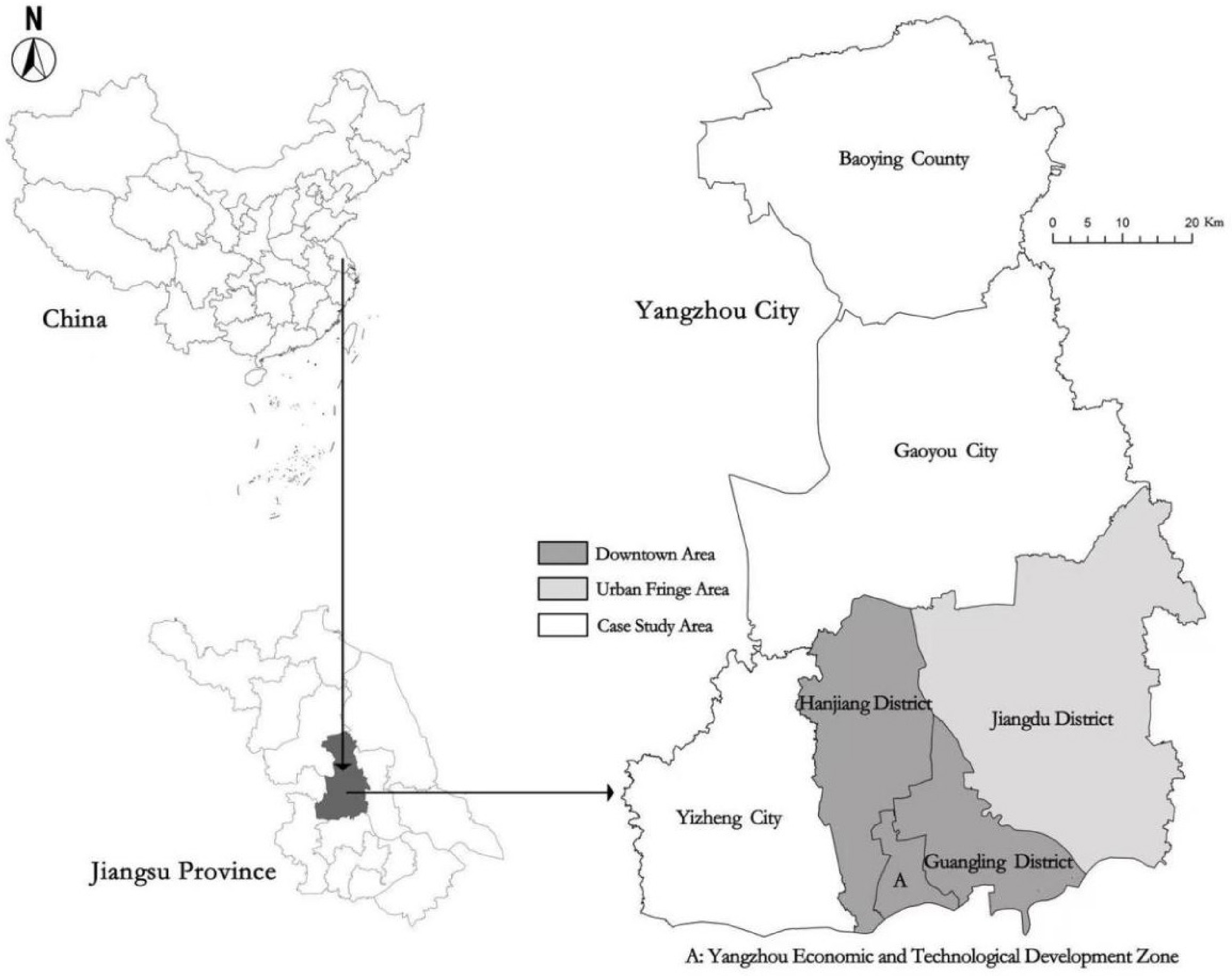
Figure 1.
Case study map of Yangzhou (Source: the authors).
-
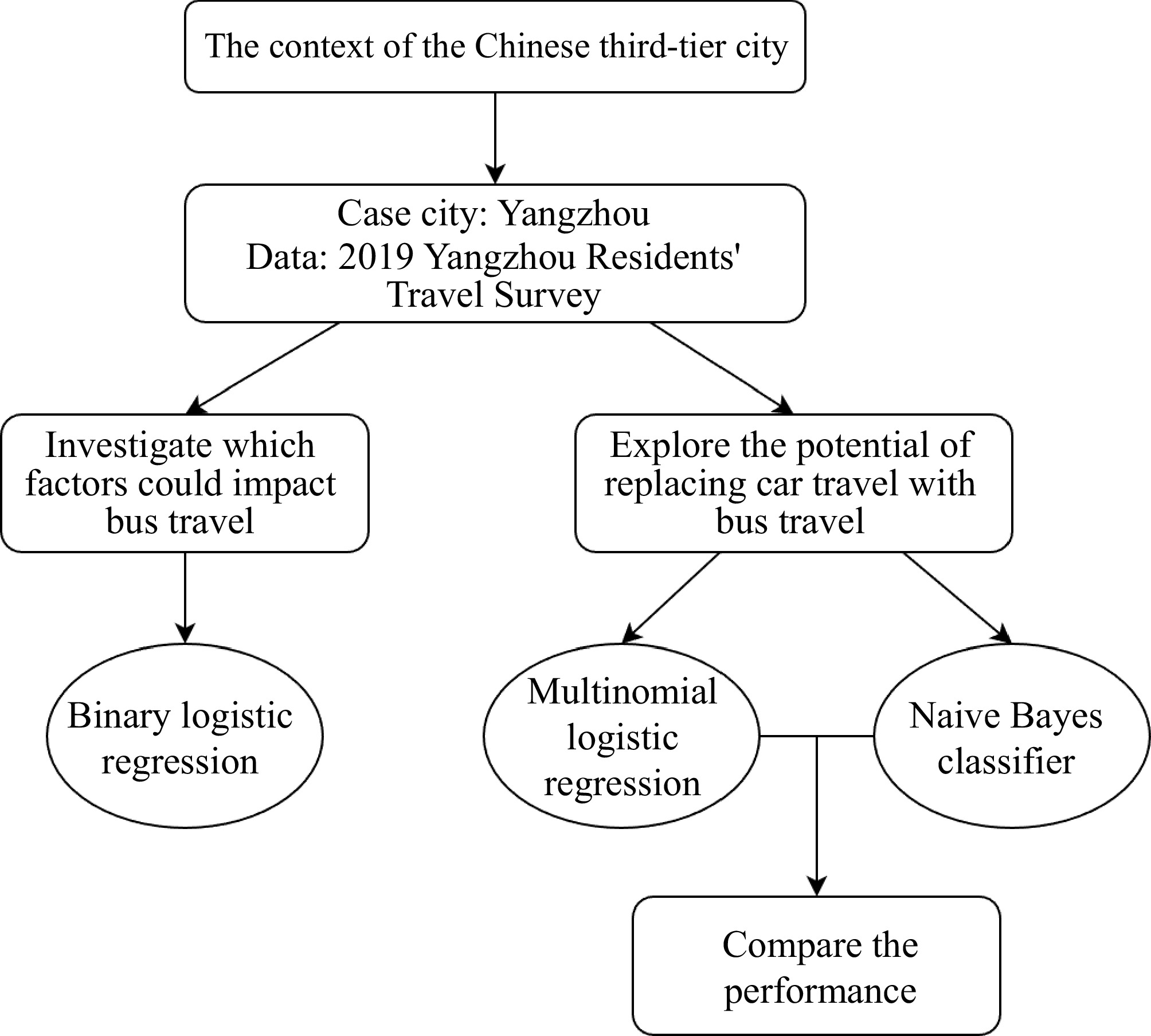
Figure 2.
Research design.
-
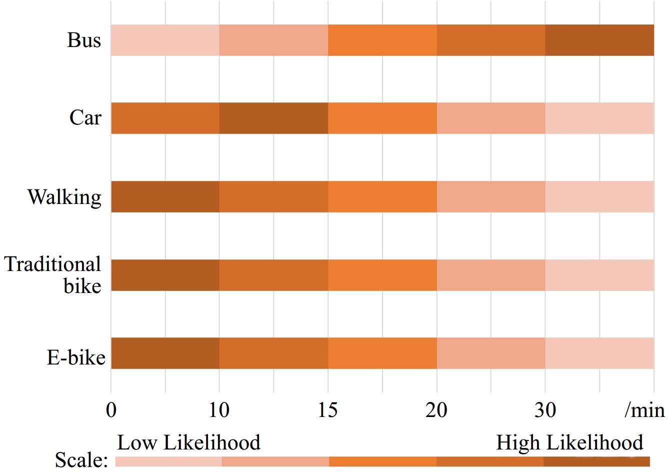
Figure 3.
The likelihood of using different transport modes for different travel times.
-
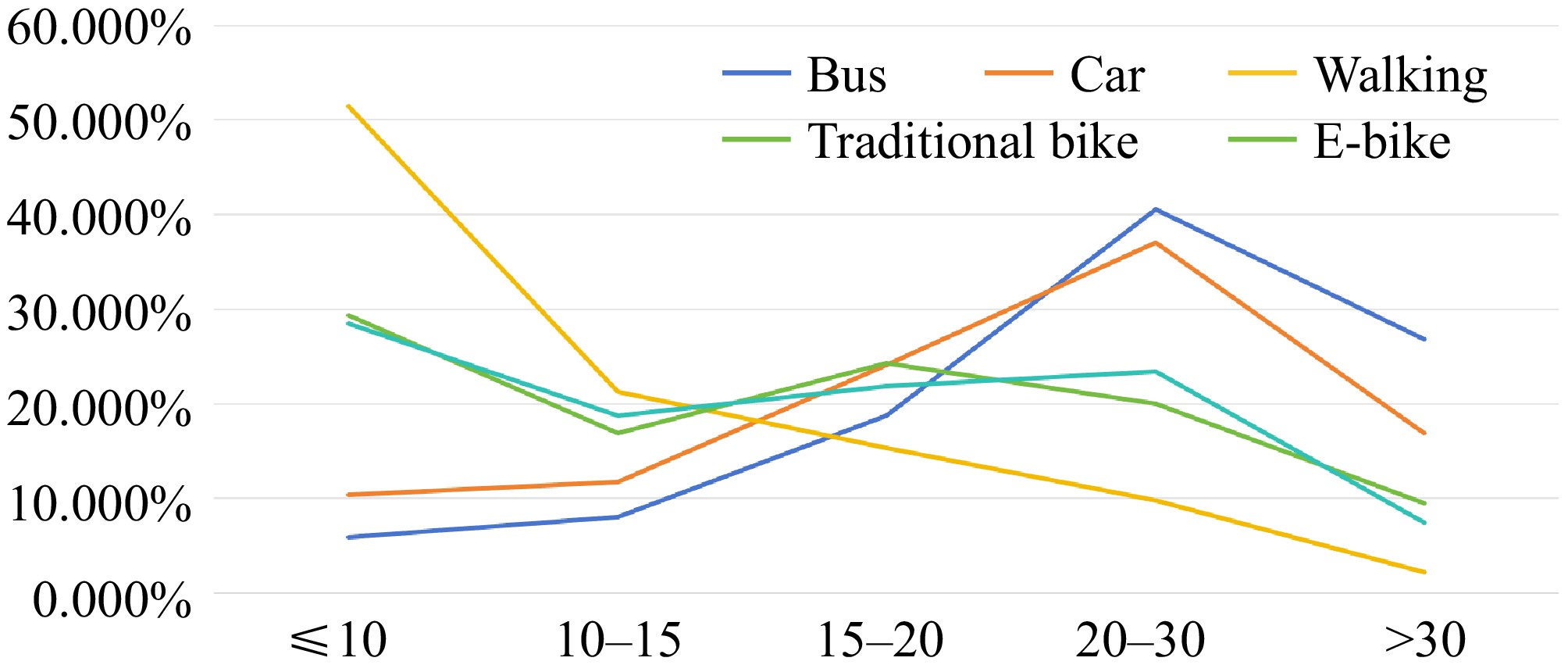
Figure 4.
The probability of using different transport modes for different travel times.
-
Types Urban permanent population Small city Type II small city < 0.2 million Type I small city > 0.2 million and < 0.5 million Medium-sized city > 0.5 million and < 1 million Large city Type II large city > 1 million and < 3 million Type I large city > 3 million and < 5 million Mega city > 5 million and < 10 million Super mega city > 10 million Source: The State Council of the PRC[33]. Table 1.
Types of Chinese cities.
-
Types Chinese cities Global cities Alpha++ / London and New York Alpha+ Chinese first-tier cities: Beijing and Shanghai E.g., Paris, Tokyo, and Sydney Alpha Chinese first-tier city: Guangzhou E.g., Los Angeles, Frankfurt, and Seoul Alpha− Chinese first-tier city: Shenzhen E.g., Brussels, Melbourne, and San Francisco Beta+ Chinese new first-tier cities: Chengdu, Tianjin, and Hangzhou E.g., Rome, Doha, and Miami Beta Chinese new first-tier cities: Chongqing, Nanjing, Wuhan, Zhengzhou, and Suzhou.
Chinese second-tier cities: Xiamen, Jinan, Shenyang, and DalianE.g., Cairo, Oslo, and Abu Dhabi Beta− Chinese new first-tier cities: Qingdao, Changsha, Xi'an, and Hefei.
Chinese second-tier city: KunmingE.g., Casablanca, Denver, and Manchester Gamma+ Chinese second-tier cities:Fuzhou and Taiyuan E.g., Austin, Rotterdam, and Adelaide Gamma Chinese new first-tier city: Ningbo. Chinese second-tier city: Harbin.
Chinese third-tier city: HaikouE.g., Osaka, Birmingham, and Detroit Gamma− Chinese second-tier cities: Nanchang and Changchun E.g., Pittsburgh, Edinburgh, and Penang High sufficiency Chinese second-tier cities: Zhuhai and Shijiazhuang E.g., Glasgow, Phoenix, and Algiers Sufficiency Chinese new first-tier cities: Wuxi and Dongguan. Chinese second-tier cities: Guiyang, Nanning, Foshan, Lanzhou, Baoding, and Wenzhou. Chinese third-tier cities: Urumqi, Hohhot, Tangshan, and Yinchuan E.g., Ottawa, Yangon, and Liverpool Source: The Rising Lab[6]; GaWC[34]. Table 2.
Comparison of Chinese and global cities.
-
Underground
constructionLight rail
constructionPublic fiscal budget revenue > 30 billion CNY > 15 billion CNY Regional GDP > 300 billion CNY > 150 billion CNY Urban permanent population > 3 million > 1.5 million Proposed initial passenger traffic intensity > 7,000 passengers per km per d > 4,000 passengers per km per d Long-term passenger flow scale > 30,000 passengers per h in one direction at peak time > 10,000 passengers per h in one direction at peak time Source: The State Council of the PRC[39] Table 3.
Standards for a city to build urban rail transit.
-
Categories Frequency Percentage Socio-demographics Gender Female 3,859 50.34% Male 3,807 49.66% Age < 25 324 4.23% 25‒34 2,117 27.62% 35‒44 2,300 30.00% 45‒54 1,462 19.07% 55‒64 884 11.53% ≥ 65 579 7.55% Annual income (CNY) ≤ 30,000 1,178 15.37% 30,000‒50,000 1,454 18.97% 50,000‒80,000 2,174 28.36% 80,000‒120,000 1,979 25.82% > 120,000 881 11.49% Living area Downtown area 6,501 84.80% Urban fringe area 1,165 15.20% Car ownership Yes 3,797 49.53% No 3,869 50.47% Whether respondents have children Yes 3,515 45.85% No 4,151 54.15% Travel behaviour Travel time (min) ≤ 10 2,085 27.20% 10‒15 1,286 16.78% 15‒20 1,628 21.24% 20‒30 1,919 25.03% > 30 748 9.76% Walking time to bus stops (min) ≤ 5 4,509 58.82% > 5 3,157 41.18% Average waiting time for buses (min) ≤ 10 6,717 87.62% > 10 949 12.38% Whether travelling in the peak period Peak period 4,967 64.79% Off-peak period 2,699 35.21% Average number of trips per day ≤ 2 4,419 57.64% > 2 3,247 42.36% Attitudes towards Yangzhou's transport system Satisfied 6,445 84.07% Unsatisfied 1,221 15.93% Transport mode Bus 409 5.34% Car 1,556 20.30% Walking 1,109 14.47% Traditional bike 228 2.97% E-bike 4,364 56.93% Table 4.
Descriptive statistics (n = 7,684).
-
Category Variable Explanation and measurement Socio-demographics Gender Binary variable (1 = male, 0 = female) Age Continuous variables Annual income Continuous variables Living area Binary variable (1 = downtown area, 0 = urban fringe area) Car ownership Binary variable (1 = yes, 0 = no) Whether respondents have children Binary variable (1 = yes, 0 = no) Travel behaviour Travel time Binary variable (1 = travel time ≤ 10 min, 0 = no) Binary variable (1 = travel time is between 10 and 15 min, 0 = no) Binary variable (1 = travel time is between 15 and 20 min, 0 = no) Binary variable (1 = travel time is between 20 and 30 min, 0 = no) Binary variable (1 = travel time > 30 min, 0 = no) Walking time to bus stops Binary variable (1 = walking time to bus stops ≤ 5 min, 0 = walking time to bus stops > 5 min) Average waiting time for buses Binary variable (1 = average waiting time for buses ≤ 10 min, 0 = average waiting time for buses > 10 min) Whether travelling in the peak period Binary variable (1 = travelling in the peak period, 0 = travelling in the off-peak period) Average number of trips per day Continuous variables Attitudes towards Yangzhou's transport system Binary variable (1 = satisfied, 0 = unsatisfied) Table 5.
Independent variables included in the models.
-
Variable B Standard error Sig. Exp(B) 95% CI for Exp(B) Lower Upper Socio-demographics Gender −0.249 0.110 0.023** 0.780 0.629 0.967 Age 0.022 0.004 0.000*** 1.022 1.014 1.030 Annual income −0.104 0.032 0.001*** 0.901 0.846 0.960 Living area 0.724 0.229 0.002*** 2.063 1.317 3.231 Car ownership −0.506 0.115 0.000*** 0.603 0.482 0.755 Whether respondents have children −0.093 0.114 0.415 0.911 0.728 1.140 Travel behaviour Walking time to bus stops 0.217 0.114 0.056* 1.242 0.994 1.552 Average waiting time for buses 0.412 0.185 0.026** 1.509 1.050 2.170 Whether travelling in the peak period −0.328 0.115 0.004*** 0.720 0.575 0.902 Average number of trips per day −0.185 0.057 0.001*** 0.831 0.742 0.930 Attitudes towards Yangzhou's transport system −0.173 0.325 0.595 0.841 0.445 1.592 Travel time (min) ≤ 10 −2.782 0.225 0.000*** 0.062 0.040 0.096 10 < x ≤ 15 −2.203 0.218 0.000*** 0.110 0.072 0.169 15 < x ≤ 20 −1.432 0.162 0.000*** 0.239 0.174 0.328 20 < x ≤ 30 −0.763 0.135 0.000*** 0.466 0.358 0.608 > 30 Control group Pseudo R2 = 0.152. The meaning of values in boldface: * p-value < 0.1, ** p-value < 0.05, *** p-value < 0.01. Table 6.
Results of the binary logistic regression (1 = travelled by bus, 0 = otherwise; n = 7,666).
-
Variable B Standard error Sig. Exp(B) 95% CI for Exp(B) Lower Upper Travel time (continuous) 0.040 0.003 0.000*** 1.041 1.034 1.048 The meaning of values in boldface: * p-value < 0.1, ** p-value < 0.05, *** p-value < 0.01. This table only shows the results for travel time, and other indicators are shown in Supplementary Table S1. Table 7.
Results of the binary logistic regression (1 = travelled by bus, 0 = otherwise; n = 7,666).
-
Categories Car Walking Traditional bike E-bike B Sig. Exp(B) B Sig. Exp(B) B Sig. Exp(B) B Sig. Exp(B) Socio-demographics Gender 1.586 0.000*** 4.883 −0.010 0.939 0.990 0.549 0.002*** 1.731 −0.080 0.478 0.923 Age −0.061 0.000*** 0.941 0.027 0.000*** 1.027 −0.007 0.276 0.993 −0.029 0.000*** 0.971 Annual income 0.519 0.000*** 1.680 −0.057 0.135 0.945 −0.198 0.000*** 0.820 0.081 0.016** 1.084 Living area −1.176 0.000*** 0.309 −1.088 0.000*** 0.337 0.038 0.910 1.039 −0.467 0.045** 0.627 Car ownership 3.654 0.000*** 38.614 −0.039 0.776 0.962 −0.107 0.561 0.898 −0.172 0.142 0.842 Whether respondents have children 0.192 0.148 1.211 −0.029 0.831 0.971 −0.346 0.067* 0.708 0.159 0.171 1.173 Travel behaviour Walking time to bus stops −0.201 0.134 0.818 −0.201 0.137 0.818 −0.008 0.967 0.992 −0.274 0.018** 0.760 Average waiting time for buses −0.539 0.011** 0.583 −0.214 0.323 0.808 0.383 0.239 1.466 −0.441 0.019** 0.643 Whether travelling in the peak period 0.240 0.085* 1.271 0.184 0.165 1.202 0.132 0.460 1.141 0.372 0.001*** 1.450 Average number of trips per day 0.086 0.197 1.090 0.320 0.000*** 1.377 0.064 0.455 1.076 0.188 0.001*** 1.207 Attitudes towards Yangzhou's transport system 0.647 0.085* 1.911 0.447 0.312 1.563 −0.183 0.729 0.833 0.003 0.992 1.003 Travel time (min) ≤ 10 1.002 0.000*** 2.724 4.134 0.000*** 62.442 2.699 0.000*** 14.861 2.779 0.000*** 16.108 10 < x ≤ 15 1.054 0.000*** 2.869 3.159 0.000*** 23.556 2.037 0.000*** 7.670 2.321 0.000*** 10.191 15 < x ≤ 20 0.947 0.000*** 2.577 2.012 0.000*** 7.482 1.543 0.000*** 4.678 1.505 0.000*** 4.504 20 < x ≤ 30 0.597 0.001*** 1.817 0.956 0.000*** 2.602 0.605 0.044** 1.831 0.852 0.000*** 2.343 > 30 Control group Pseudo R2 = 0.537. The meaning of values in boldface: * p-value < 0.1, ** p-value < 0.05, *** p-value < 0.01. Table 8.
Results of the multinomial logistic regression (n = 7,666).
-
Travel time (min) Likelihood ranking Bus Car Walking Traditional bike E-bike 1 > 30 10 < x ≤ 15 ≤ 10 ≤ 10 ≤ 10 2 20 < x ≤ 30 ≤ 10 10 < x ≤ 15 10 < x ≤ 15 10 < x ≤ 15 3 15 < x ≤ 20 15 < x ≤ 20 15 < x ≤ 20 15 < x ≤ 20 15 < x ≤ 20 4 10 < x ≤ 15 20 < x ≤ 30 20 < x ≤ 30 20 < x ≤ 30 20 < x ≤ 30 5 ≤ 10 > 30 > 30 > 30 >3 0 In this table, the results for bus travel were from Section Binary logistic regression; the results for car, walking, traditional bike, and e-bike travel were from Section Multinomial logistic regression. Table 9.
The rank of the likelihood of using different transport modes for different travel times.
-
Travel time (min) Probability Bus Car Walking Traditional bike E-bike ≤ 10 5.93% 10.32% 51.50% 29.38% 28.52% 10−15 8.05% 11.74% 21.28% 16.91% 18.73% 15−20 18.70% 24.07% 15.32% 24.26% 21.82% 20−30 40.51% 37.03% 9.75% 19.96% 23.45% > 30 26.81% 16.85% 2.15% 9.48% 7.48% Total 100.00% 100.00% 100.00% 100.00% 100.00% The values in boldface represent the highest probability of using the bus and car for different travel times. Table 10.
The probability of using different transport modes for different travel times via Naive Bayes.
-
Bus Car Walking Traditional
bikeE-bike Accuracy Naive Bayes classifiers 0.37 0.33 0.59 0.33 0.34 Multinomial logistic regression 0.22 0.25 0.20 0.17 0.12 DIC Naive Bayes classifiers 226.43 934.06 512.49 139.42 2,577.18 Multinomial logistic regression 13,087.62 Table 11.
Comparison of the performance between multinomial logistic regression and Naive Bayes classifier.
-
Travel time (min) Probability ranking Bus Car Walking Traditional bike E-bike 1 20 < x ≤ 30 20 < x ≤ 30 ≤ 10 ≤ 10 ≤ 10 2 > 30 15 < x ≤ 20 10 < x ≤ 15 15 < x ≤ 20 20 < x ≤ 30 3 15 < x ≤ 20 > 30 15 < x ≤ 20 20 < x ≤ 30 15 < x ≤ 20 4 10 < x ≤ 15 10 < x ≤ 15 20 < x ≤ 30 10 < x ≤ 15 10 < x ≤ 15 5 ≤ 10 ≤ 10 > 30 > 30 > 30 Table 12.
The rank of the probability of using different transport modes for different travel times.
Figures
(4)
Tables
(12)