


-
The role of transport in driving the rapid development of Chinese cities has aroused great interest among scholars worldwide[1]. Although previous studies distilled the key messages from the rich set of resources and reflected the diversity of China to some extent, these studies were primarily dominated by more prestigious Chinese first-tier (Beijing, Shanghai, Guangzhou, and Shenzhen), new first-tier (e.g., Xi'an and Suzhou), or second-tier cities (e.g., Shenyang and Ji'nan). However, Chinese third-tier cities have been neglected. Prestigious media and academic institutions have primarily paid attention to Chinese first-tier cities, new first-tier cities, and second-tier cities, and few studies by Chinese or worldwide scholars use 'Chinese third-tier city' and 'transport' as keywords. There are only four first-tier cities, 15 new first-tier cities, and 30 second-tier cities, but there are 70 third-tier cities[2−6]. Chinese third-tier cities, as typical developing cities in China, usually have between half a million and 3 million urban permanent residents per city. Given that there are 70 third-tier cities out of 337 cities in China, on the one hand, Chinese third-tier cities occupy a large proportion of the national land area; on the other hand, they have a large population, with more than 84 million urban permanent residents and more than 365 million total permanent residents[7]. Compared with more developed Chinese first-tier cities, new first-tier cities, and second-tier cities, Chinese third-tier cities usually only have buses as public transport. Therefore, policy implications derived from previous studies may not be relevant to these cities.
Although the aim worldwide is to provide better public transport services to encourage public transport use and then reduce traffic congestion[8], the potential of public transport to reduce congestion has not yet been fully realised[9]. In addition, the increase in carbon emissions has accelerated climate change and threatened the cities' sustainable development. Yet, with the rapid growth of private vehicles, controlling CO2 emissions produced by transport has become increasingly difficult[10]. To set up a resource-conserving and environmentally friendly society, public transport priority, as one of the Travel Demand Management (TDM) strategies, has been generally regarded as an essential measure to tackle issues in cities' sustainable development, such as traffic congestion and pollution, by scholars and practitioners[8−12]. Accordingly, China has introduced a series of transportation policies at the national level to reduce car ownership and prioritise public transport, summarised as follows[10]: China formally proposed the public transport priority policy in 2004 and re-emphasised the public transport priority policy as the national strategy in 2012; in 2023, China required public transport priority policy to continue to be implemented; among them, the construction of bus transport is the main body to realise prioritising public transport, especially in the context of recently limited fiscal funds and an aging population. As a result, in China, between 2004 and 2017, the length of bus routes increased fivefold, and the number of buses doubled[13]. However, from 2003 to 2013, the number of private cars increased 13 times[14]; in 2018, car ownership in China exceeded 200 million[15].
Traffic congestion also has been expanded to Chinese third-tier cities[16], and car ownership in some of them has exceeded 2 million, and even 3 million[17]. As public transport in Chinese third-tier cities usually only have buses, the development of bus travel plays a vital role. Liu et al.[9] summarised that current studies focussing on bus travel can be roughly divided into two types: the first type concentrated on investigating factors affecting bus use[12,18−27], and the second type concentrated on exploring the relationship between car ownership and bus use[8,28−32]. Although some studies have considered the relationship between car ownership or car use and bus travel[8,12], few have examined the influence of other transport modes simultaneously, such as walking and cycling[9]. Additionally, few studies have compared the likelihood of using buses and other transport modes at different travel times[9]. Among the existing literature, only a study from Liu et al.[9], based on a Chinese third-tier city, Heze tried to fill in these blanks. However, only one empirical study might not reflect the overall transport situation of 70 Chinese third-tier cities.
To address the above research gaps, this study is based on Yangzhou, another Chinese third-tier city. It used data from the 2019 Yangzhou Residents' Travel Survey to adopt binary logistic regression to investigate which factors could impact bus travel, and it adopted multinomial logistic regression and the Naive Bayes algorithm to explore the potential of replacing car travel with bus travel.
-
In 2014, The State Council of the PRC, taking the urban permanent population as its statistical reference divided Chinese cities into seven types, as shown in Table 1. According to the 2020 Chinese Census (Seventh National Population Census), there are 575 million urban permanent residents, which account for more than 63% of the non-rural permanent population (902 million) and 40.8% of the total population (1.41 billion)[7]. Since the urban permanent population is the only indicator, this kind of city classification method may not reflect cities' comprehensive strengths.
Table 1. Types of Chinese cities.
Types Urban permanent population Small city Type II small city < 0.2 million Type I small city > 0.2 million and < 0.5 million Medium-sized city > 0.5 million and < 1 million Large city Type II large city > 1 million and < 3 million Type I large city > 3 million and < 5 million Mega city > 5 million and < 10 million Super mega city > 10 million Source: The State Council of the PRC[33]. Types of Chinese cities classified by scholars and institutions
-
The Rising Lab is a journalism program focusing on business data under the Yicai Media Group; as an authority in China, The Rising Lab has established a Ranking of Cities' Business Attractiveness in China annually. The Rising Lab[2−6] applies a comprehensive framework with various indicators to quantitatively evaluate cities based on their performance in the previous year. It is noted that indicators directly related to urban transport account for around 20% of total impacts. Correspondingly, the ranking of cities and the tier of some cities will change yearly, potentially encouraging cities' development. According to each city's score from high to low, it annually evaluates four first-tier cities, 15 new first-tier cities, 30 second-tier cities, 70 third-tier cities, 90 fourth-tier cities, and 128 fifth-tier cities. Since most have urban permanent populations between 0.5 million and 3 million, Chinese third-tier cities primarily belong to Type II large cities and medium-sized cities[6,7,33].
Combining the latest annual ranking report from The Rising Lab[6], the city classification from The State Council of the PRC[33], and the population information in the Tabulation on 2020 China Population Census by County from The State Council of the PRC[7], Chinese first-tier cities have an urban permanent population of about 70 million and a total population of about 83 million; the new first-tier cities have an urban permanent population of about 118 million and a total population of about 195 million; the second-tier cities have an urban permanent population of about 101 million and a total population of about 224 million; the third-tier cities have an urban permanent population of about 84 million and a total population of about 365 million. Then, the ratio of the urban permanent population to the total population of each tier of cities could be calculated, the results are as follows: first-tier cities (84.34%), new first-tier cities (60.51%), second-tier cities (45.09%), and third-tier cities (23.01%), which might reflect that Chinese third-tier cities have a lower urbanisation rate than first-tier, new first-tier, or second-tier cities. In other words, Chinese first-tier, new first-tier, and second-tier cities are more developed than third-tier cities.
The Rising Lab's city classification only focuses on Chinese cities. Thus, comparing Chinese cities with global ones is necessary through the prestigious global city classification or ranking method. For example, the latest release, The World According to GaWC 2024, produced by Globalization & World Cities (GaWC)[34], classified cities into Alpha++, Alpha+, Alpha, Alpha−, Beta+, Beta, Beta−, Gamma+, Gamma, Gamma−, High Sufficiency, and Sufficiency cities, which involved 42 of 337 Chinese cities evaluated by The Rising Lab, as shown in Table 2.
Table 2. Comparison of Chinese and global cities.
Types Chinese cities Global cities Alpha++ / London and New York Alpha+ Chinese first-tier cities: Beijing and Shanghai E.g., Paris, Tokyo, and Sydney Alpha Chinese first-tier city: Guangzhou E.g., Los Angeles, Frankfurt, and Seoul Alpha− Chinese first-tier city: Shenzhen E.g., Brussels, Melbourne, and San Francisco Beta+ Chinese new first-tier cities: Chengdu, Tianjin, and Hangzhou E.g., Rome, Doha, and Miami Beta Chinese new first-tier cities: Chongqing, Nanjing, Wuhan, Zhengzhou, and Suzhou.
Chinese second-tier cities: Xiamen, Jinan, Shenyang, and DalianE.g., Cairo, Oslo, and Abu Dhabi Beta− Chinese new first-tier cities: Qingdao, Changsha, Xi'an, and Hefei.
Chinese second-tier city: KunmingE.g., Casablanca, Denver, and Manchester Gamma+ Chinese second-tier cities:Fuzhou and Taiyuan E.g., Austin, Rotterdam, and Adelaide Gamma Chinese new first-tier city: Ningbo. Chinese second-tier city: Harbin.
Chinese third-tier city: HaikouE.g., Osaka, Birmingham, and Detroit Gamma− Chinese second-tier cities: Nanchang and Changchun E.g., Pittsburgh, Edinburgh, and Penang High sufficiency Chinese second-tier cities: Zhuhai and Shijiazhuang E.g., Glasgow, Phoenix, and Algiers Sufficiency Chinese new first-tier cities: Wuxi and Dongguan. Chinese second-tier cities: Guiyang, Nanning, Foshan, Lanzhou, Baoding, and Wenzhou. Chinese third-tier cities: Urumqi, Hohhot, Tangshan, and Yinchuan E.g., Ottawa, Yangon, and Liverpool Source: The Rising Lab[6]; GaWC[34]. In total, The World According to GaWC 2024[34] concentrated on more developed Chinese cities, including all four first-tier cities, all 15 new first-tier cities, and 18 of 30 second-tier cities; however, only five third-tier cities, and none of the fourth-tier and fifth-tier cities were involved. As mentioned, most existing studies have primarily focused on the more developed Chinese first-tier, new first-tier, or second-tier cities, while third-tier cities have been neglected. On the one hand, although some prestigious media (e.g., CCTV[35] and China Daily[36]), and academic institutions (e.g., Urban Planning Society of China[37]) reprint or refer to The Rising Lab's city classification and the relevant rank, they have primarily focused on Chinese first-tier cities, new first-tier cities, and second-tier cities rather than third-tier cities. On the other hand, after searching academic publications within China National Knowledge Infrastructure (CNKI), few studies by Chinese or worldwide scholars use 'Chinese third-tier city' and 'transport' as keywords. Compared with more developed cities, the transport situation in Chinese third-tier cities is unique because buses are usually the only public transport form, which will be discussed in the following section.
Public transport in Chinese third-tier cities
-
The Ministry of Transport of the PRC[38] reported that as of December 2023, urban rail transit systems were in operation in 55 cities (containing three county cities) in mainland China. All Chinese first-tier and new first-tier cities have operated urban rail transit; 73.3% of second-tier cities have operated urban rail transit; only seven third-tier cities have operated urban rail transit[6,38]. Among these Chinese third-tier cities with urban rail transit (i.e., Hohhot, Wuhu, Luoyang, Urumqi, Huai'an, Xianyang, and Sanya), Hohhot and Urumqi are two provincial capital cities; Luoyang, Xianyang, and Sanya are famous tourist cities. Therefore, typical Chinese third-tier cities hardly have any urban rail transit and only have bus transport as the public transport.
In China, the standard for a city to build urban rail transit is the "Opinions on Further Strengthening the Planning, Construction and Management of Urban Rail Transit" issued by the State Council of the PRC[39] in July 2018, as shown in Table 3. All proposed construction of urban rail transit should follow the standard.
Table 3. Standards for a city to build urban rail transit.
Underground
constructionLight rail
constructionPublic fiscal budget revenue > 30 billion CNY > 15 billion CNY Regional GDP > 300 billion CNY > 150 billion CNY Urban permanent population > 3 million > 1.5 million Proposed initial passenger traffic intensity > 7,000 passengers per km per d > 4,000 passengers per km per d Long-term passenger flow scale > 30,000 passengers per h in one direction at peak time > 10,000 passengers per h in one direction at peak time Source: The State Council of the PRC[39] Currently, it is difficult for Chinese third-tier cities to reach these requirements even though some local governments have set up relevant urban transit rail planning[40]. On the one hand, the population of the central urban areas of most third-tier cities grows relatively slowly, and there may even be population outflow. On the other hand, from the perspective of industrial structure, although the total economic volume and fiscal revenue of some third-tier cities are relatively high, the cities dominated by industry have much smaller passenger flows than those dominated by the service industry, and the demand for urban rail transit is also much lower. Given that urban rail transit in most Chinese third-tier cities is almost impossible to build in the short term, the development of bus transport is an essential focus that should be considered to improve the transport of Chinese third-tier cities.
Factors affecting bus travel
-
Over the past seven decades, researchers have continuously investigated the factors that impact travel behaviour and transport mode choices[41]. Socio-demographic factors could affect the use of public transport. Several existing studies have indicated that young (under 25 years old) and older adults are more likely to use public transport[9,22,23,25,42,43]; in comparison, middle-aged people seem to be more dependent on cars[22]. An association between gender and public transport use has been found; studies by Buehler[19], and Ng & Acker[24] demonstrated that females are more likely to use public transport than males. Also, those facing financial stress, such as the unemployed, tend to travel by bus[8,9].
Higher levels of accessibility can increase public transport use[12,22]. Litman[44] defined bus accessibility as containing several factors: access to bus stops, travel time by bus, bus frequency, and ticket prices. Rasca & Saeed[12] found that a longer distance to the nearest bus stop negatively impacts bus use. They also found that travellers living within a comfortable walking distance of bus stops (e.g., five minutes or less) are more willing and likely to travel by bus. Furthermore, numerous studies, such as a study from Brechan[18] explored 24 experimental cases in Norway, and found that reducing prices and increasing the frequency of buses can attract public transport use[12,23,26,28]. Travel time is another key point that needs to be considered for public transport. Some studies claimed that very long travel times harm public transport use[23,28,45]. By comparing bus travellers with different travel times, Rasca & Saeed[12] found a threshold effect: when travel time is between 15 and 60 min, respondents are more likely to travel by bus as the travel time increases, while when travel time is over 60 min, respondents are least likely to travel by bus. However, Liu et al.[9], through an empirical study based in a Chinese third-tier city, Heze proved that respondents are more likely to travel by bus with travel time increases.
Car travel vs public transport travel
-
With the rapid development of the economy and urbanization in China, Chinese second-tier and third-tier cities have gradually obtained large-scale development, which also increased traffic pressure and expanded traffic congestion from developed cities to developing cities[16]. Although Chinese third-tier cities are not as developed as first-tier, new first-tier, or second-tier cities, the number of cars in some third-tier cities has exceeded 2 million and even 3 million[17]. Besides the rapid growth of car ownership and car use, Sun et al.[46], and Wang[16] summarised other causes of urban traffic congestion. They indicated that insufficient public transport infrastructure and inadequate services lead to the disadvantaged development of public transport, which is one of the key reasons for congestion.
Existing research has produced evidence that higher car ownership has adverse effects on the use of public transport (e.g., bus)[12,21,26,28,47]. In turn, better quality of bus services significantly negatively impacts car ownership[8,31,32, 48,49] and leads to an increase in bus use and a reduction in car use[8,30–32]. For example, based on surveying car commuters in Shanghai, Wang et al.[50] found that improving the punctuality and comfort of public transport could reduce car use. Several studies investigating car users' subjective attitudes found that improving bus services may lead to travellers having a more positive attitude towards bus travel and a more negative attitude towards car travel[51−54]. Also, faster public transport services could encourage car users to use public transport[55]. Kingham et al.[53] stated that enhancing bus service (e.g., reliability, convenience, and connections) and offering discounted tickets could switch 40% of car commuters to buses. Furthermore, travellers with financial constraints tend to travel by bus[8], as discussed in the previous section. Conversely, car ownership and use generally increase with income[8,56,57].
Travel time could reflect the competition between public transport and car travel[23]. During the peak period, public transport may offer shorter travel time than cars, while during the off-peak period, the opposite is true[23,58]. However, Kawabata[45] discovered that commuters who travelled by car had much higher job accessibility for a 30-min threshold than those who travelled by public transport. Collins & Chambers[59] found that when the travel time of a journey for public transport is 1.25 times or longer than car travel, people are significantly less willing to use public transport.
-
Yangzhou, located in the middle of Jiangsu Province, China, was chosen as a case city. The administrative planning region of Yangzhou consists of three districts, one county, two county-level cities, and one development zone, with a total land area of 6,591 km2. According to the 2020 Chinese Census (Seventh National Population Census), Yangzhou had 4.56 million permanent residents and 1.51 million urban permanent residents, with a 71.0% urbanization rate, evaluated as a Type II large city[7]. According to The Rising Lab's latest 5-year annual reports[2−6], Yangzhou was evaluated as a Chinese third-tier city and ranked among the top third-tier cities. Compared with Heze, chosen as the case city by Liu et al.[9], even though Heze has a much larger area and permanent population, Yangzhou has a larger urban permanent population, higher regional GDP, GDP per capita, and rank of cities than Heze.
In 2016, the Yangzhou Natural Resources and Planning Bureau proposed building a bus-dominated development model, which pointed out Yangzhou's future direction of transport development. According to the 2020 Annual Report on Urban Transport Development in Yangzhou, established by the Yangzhou Natural Resources and Planning Bureau[60], until the end of 2019, 3,108 buses and 245 bus routes were in operation in Yangzhou. The total length of operating routes was 5,026.4 km. The total bus passenger volume in Yangzhou was 229 million, with an average daily passenger volume of 628,300 people. Also, as of the end of 2019, Yangzhou's central urban area has built three bus lanes with a total mileage of 43.9 km, namely Wenchang Road Bus Lane, Hanjiang Road Bus Lane, and Southern Expressway Bus Lane, while only the Wenchang Road Bus Lane is in operation. In addition, until the end of 2019, there were 732,500 private cars in Yangzhou, more than 230 times the number of buses.
The analysis and discussion of this study mainly focus on the downtown area and urban fringe area, including Hanjiang District, Guangling District, Jiangdu District, and Yangzhou Economic and Technological Development Zone, as shown in Fig. 1.
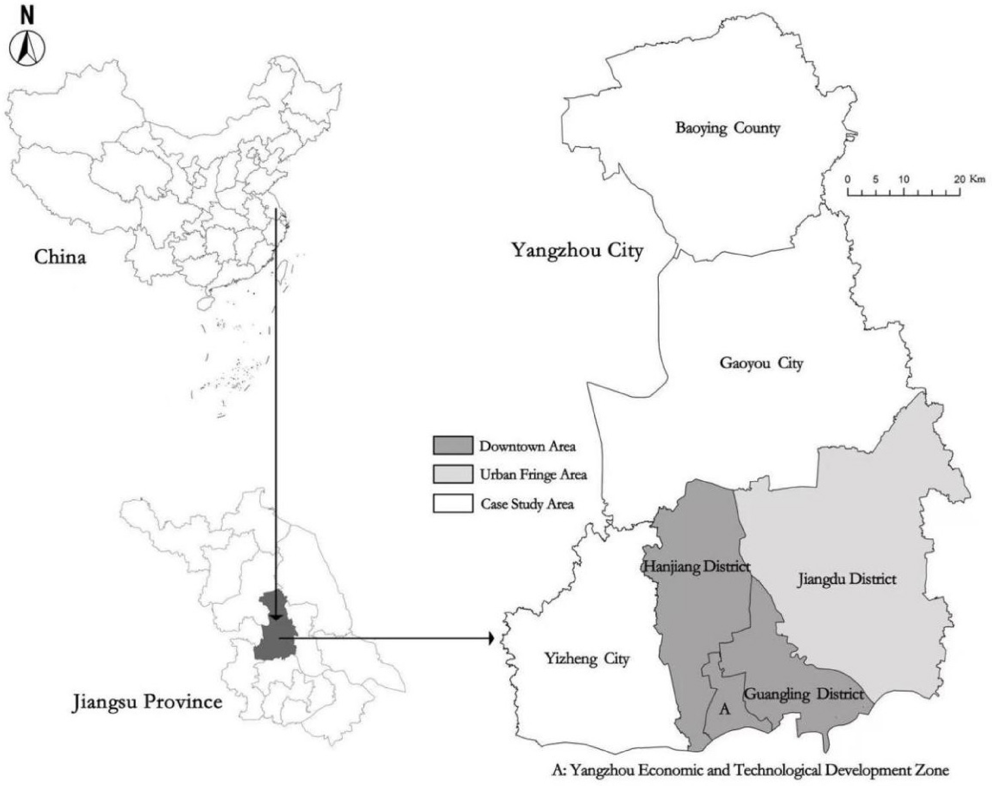
Figure 1.
Case study map of Yangzhou (Source: the authors).
Data description
-
This study adopted secondary data from the 2019 Yangzhou Residents' Travel Survey. The Yangzhou Natural Resources and Planning Bureau collected individuals' socio-demographics and residents' travel behaviour by using structured questionnaires. There were three methods adopted to ensure the representativeness of the sample: 1) randomly selecting respondents from each sub-district according to their population; 2) the sub-district with a higher population having a larger sample size; and 3) distributing paper questionnaires to people residing in each stratum. The Bureau staff members distributed these questionnaires in 2019, and respondents could contact staff members whenever necessary. All the information and data used in this study included the following 13 categories from every respondent, which could be divided into socio-demographics and travel behaviour, as shown in Table 4.
Table 4. Descriptive statistics (n = 7,684).
Categories Frequency Percentage Socio-demographics Gender Female 3,859 50.34% Male 3,807 49.66% Age < 25 324 4.23% 25‒34 2,117 27.62% 35‒44 2,300 30.00% 45‒54 1,462 19.07% 55‒64 884 11.53% ≥ 65 579 7.55% Annual income (CNY) ≤ 30,000 1,178 15.37% 30,000‒50,000 1,454 18.97% 50,000‒80,000 2,174 28.36% 80,000‒120,000 1,979 25.82% > 120,000 881 11.49% Living area Downtown area 6,501 84.80% Urban fringe area 1,165 15.20% Car ownership Yes 3,797 49.53% No 3,869 50.47% Whether respondents have children Yes 3,515 45.85% No 4,151 54.15% Travel behaviour Travel time (min) ≤ 10 2,085 27.20% 10‒15 1,286 16.78% 15‒20 1,628 21.24% 20‒30 1,919 25.03% > 30 748 9.76% Walking time to bus stops (min) ≤ 5 4,509 58.82% > 5 3,157 41.18% Average waiting time for buses (min) ≤ 10 6,717 87.62% > 10 949 12.38% Whether travelling in the peak period Peak period 4,967 64.79% Off-peak period 2,699 35.21% Average number of trips per day ≤ 2 4,419 57.64% > 2 3,247 42.36% Attitudes towards Yangzhou's transport system Satisfied 6,445 84.07% Unsatisfied 1,221 15.93% Transport mode Bus 409 5.34% Car 1,556 20.30% Walking 1,109 14.47% Traditional bike 228 2.97% E-bike 4,364 56.93% (1) Social-demographics: gender, age, annual income, living area, car ownership, and whether respondents have children.
(2) Travel behaviour: travel time, walking time to bus stops, average waiting time for buses, whether travelling in the peak period (peak periods were defined as 7:00–9:00 and 17:00–19:00, and all other periods were off-peak), the average number of trips per day, attitudes towards Yangzhou's transport system, and transport mode (bus, car, walking, traditional bikes, e-bike).
This survey's sample size is 11,901; after the authors' data cleaning, the valid sample size is 7,666, comprising 3,807 men and 3,859 women. In this study, the rule of data cleaning is that if a sample had missing information, it would be removed. In other words, the valid sample should contain all the information on the variables involved in the corresponding analysis. The gender composition of the valid sample (i.e., males accounted for 49.66%, and females accounted for 50.34%) is in line with that of Yangzhou's population based on the 2020 Chinese census (i.e., males accounted for 49.80%, and females accounted for 50.20%), which reflects a good representation of the adopted data to avoid obvious bias[61]. A very high proportion (88.51%) of the respondents were less or equal to the GDP per capita (CNY 120,000 or less), while only 11.49% had an annual income of more than CNY 120,000. The majority (84.80%) of respondents were living in the downtown area. The proportion of respondents who owned a car (49.53%) is almost equal to that of those who did not (50.47%), and the proportion of respondents who have children (45.85%) is nearly equal to that of those who have not (54.15%).
Concerning travel behaviour variables, 27.20% of the respondents average travel time for a journey lasting 10 min or less, 25.03% for a journey lasting 20 to 30 min, and 21.24% for a journey lasting 15 to 20 min, accounting for the three largest proportions. Out of all the transport modes, the number of respondents who used buses accounted for only 5.34% of the total, but it is still more than respondents who travelled by traditional bikes (2.97%). Respondents who travelled by e-bikes held the largest proportion (56.93%), followed by respondents who travelled by car (20.30%) and respondents who travelled by walking (14.47%). In metropolises, longer commuting distances made e-bikes less competitive than public transport; in contrast, relatively smaller cities attracted more e-bike usage[62]. E-bikes account for a large portion of residents' total transport modes in urban areas[60], which is another typical characteristic of Chinese third-tier cities' transport situation. By the end of 2019, Yangzhou had more than 5.5 million e-bikes, 2.85 million of which were inside the urban area[63]; the average household owned 0.51 traditional bikes and 1.73 e-bikes[60]. Compared with another statistic from the Yangzhou Natural Resources and Planning Bureau[60], in the central urban area, the proportion of bus travel was 10.63% and walking accounted for 14.73%, similar to car travel (13.16%). Cycling (traditional bikes and e-bikes) was dominant, accounting for 56.78% of all transport modes. It is noted that the above statistics only focused on the central urban area, while the 2019 Yangzhou Residents' Travel Survey involved downtown and urban fringe areas. Furthermore, the 2019 Yangzhou Residents' Travel Survey involved travel purposes of respondents not only commuting (e.g., going to work, going to school, and going to business) but also leisure (e.g., shopping, entertainment, and visiting friends).
Research method
Logistic regression
-
Logistic regression is one of the most popular methods used in the transport field, especially in analysing individuals' travel behaviour and transport mode choices[9,12]. The following studies have used binary logistic regression: Chakrabarti & Joh[20], Collins & Chambers[59], Ha et al.[23], and Liu et al.[9]; other logistic regression models adopted in existing studies include: ordered logistic regression[12] and multinomial logistic regression[9,21,25]. Liu et al.[9], and Rasca & Saeed[12] used logistic regression to explore the impacts of individual factors on bus use and investigate the likelihood of travelling by bus at different times and over different distances. This study used binary logistic regression to analyse the relationship between individual factors (i.e., socio-demographics and travel behaviour) and bus use and multinomial logistic regression to compare the likelihood of respondents using different transport modes at different travel times. The formulas are shown in the Supplementary File 1.
In the binary logistic regression model, the dependent variable is a dummy variable where 1 represents the decision to travel by bus, and 0 represents the decision not to travel by bus. Twelve independent variables related to socio-demographics (gender, age, annual income and living area, car ownership, and whether respondents have children), and travel behaviour (travel time, walking time to bus stops, average waiting time for buses, whether travelling in the peak period, average number of trips per day, and attitudes towards Yangzhou's transport system) were examined.
Given its capability to realistically reflect respondents' choice behaviour, the multinomial logistic model has dominated travel behaviour research since the 1970s[64]. Correspondingly, Mahdi & Esztergár-Kiss[65] summarised that previous studies have widely applied the multinomial logistic model to analyse travel mode choice. Because this study also aimed to explore how travel time is associated with the transport mode choice, it ran the multinomial logistic model. The multinomial logistic model contained 12 independent variables related to socio-demographics and travel behaviour, similar to the binary logistic regression model. The difference is that the dependent variable is different transport modes (bus, car, walking, traditional bike, and e-bike). More details are shown in the following sections.
Based on the descriptive statistics, Table 5 shows the variables and corresponding measurements that were the independent variables analysed in the binary and multinomial logistic regression models. In the binary logistic regression model, except for age, a continuous variable, the other variables were all binary. Multinomial logistic models were run to explore how travel time influences the choice of transport mode. When analysing the relationship between travel time and the choice of transport mode, travel time was regarded as a categorical variable containing five categories referring to Liu et al.[9]: (1) travel time ≤ 10 min, (2) travel time is between 10 and 15 min, (3) travel time is between 15 and 20 min, (4) travel time is between 20 and 30 min, and (5) travel time > 30 min.
Table 5. Independent variables included in the models.
Category Variable Explanation and measurement Socio-demographics Gender Binary variable (1 = male, 0 = female) Age Continuous variables Annual income Continuous variables Living area Binary variable (1 = downtown area, 0 = urban fringe area) Car ownership Binary variable (1 = yes, 0 = no) Whether respondents have children Binary variable (1 = yes, 0 = no) Travel behaviour Travel time Binary variable (1 = travel time ≤ 10 min, 0 = no) Binary variable (1 = travel time is between 10 and 15 min, 0 = no) Binary variable (1 = travel time is between 15 and 20 min, 0 = no) Binary variable (1 = travel time is between 20 and 30 min, 0 = no) Binary variable (1 = travel time > 30 min, 0 = no) Walking time to bus stops Binary variable (1 = walking time to bus stops ≤ 5 min, 0 = walking time to bus stops > 5 min) Average waiting time for buses Binary variable (1 = average waiting time for buses ≤ 10 min, 0 = average waiting time for buses > 10 min) Whether travelling in the peak period Binary variable (1 = travelling in the peak period, 0 = travelling in the off-peak period) Average number of trips per day Continuous variables Attitudes towards Yangzhou's transport system Binary variable (1 = satisfied, 0 = unsatisfied) Naive Bayes classifier
-
In addition to the popular logistic regression model, Bayesian methods have presented good prediction accuracy and performance[66−70]. Many previous empirical studies have adopted various Bayesian models to analyse travel mode choices, such as the Bayesian binary logistic model[71], Bayesian multinomial logistic model[68], and Bayesian network[72]. Among them, Naive Bayes has been paid widespread attention when comparing traditional logistic regression and machine learning methods[64,65,73]. As a powerful probabilistic classifier for predictive modelling based on Bayes theorem, Naive Bayes has the following advantages: (1) its prediction criteria are simple; (2) it performs well for binary and multi-class classification[74,75]. Although the Naive Bayes classifier is a relatively simple machine learning method for calculating class probabilities, it has been proven more competitive than other advanced classifiers, such as decision trees[76]. The mathematical expression for Bayes theorem has been shown in the Supplementary File 1. To validate the fitness of the multinomial logistic regression, this study also adapted the Naive Bayes classifier to explore how travel time influences the choice of transport mode. Five Naive Bayes classifiers were conducted to analyse five different transport modes to output probabilities of using the corresponding transport modes for different travel times. Different from the binary and multinomial logistic regressions discussed above, in these five Naive Bayes classifiers, three continuous variables in Table 5 (i.e., age, annual income, and the average number of trips per day) were regarded as categorical variables, and the classification of these three variables are identical to those in Table 4.
Referring to Xiao et al.[77], and Yuan et al.[78], for model comparison, the Deviance Information Criterion (DIC) is applied to compare the models[79−81]:
$ DIC=D\left(\bar{\theta }\right)+2{p}_{D}=\bar{D}+{p}_{D} $ where,
$ D(\bar{\theta }) $ $ \bar{\theta } $ $ {p}_{D} $ $ \bar{D} $ $ D(\bar{\theta }) $ According to the above description and discussion, Fig. 2 presents the research design of this study.
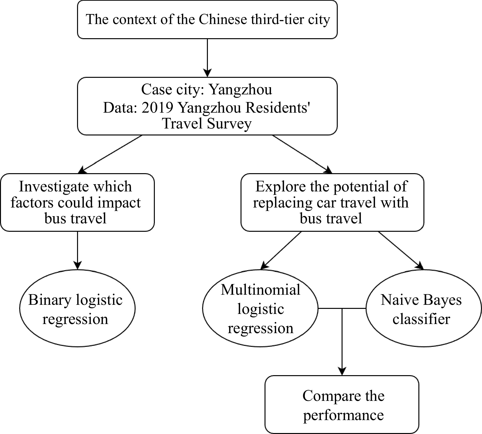
Figure 2.
Research design.
-
Before all of the analyses, referring to the study by Cheng et al.[82], and Rasca & Saeed[12], a variance inflation factor (VIF) analysis was performed to detect possible multicollinearity among the independent variables. All the socio-demographics and travel behaviour variables in Table 5 have a VIF value of less than five; thus, they are retained in the subsequent analysis.
Table 6 shows the binary logistic regression results for the impacts of socio-demographics and travel behaviour factors on the bus travel decision, which was significantly influenced by the following 10 factors: gender (p = 0.023 < 0.05), age (p = 0.000 < 0.01), annual income (p = 0.001 < 0.01), living area (p = 0.002 < 0.01), car ownership (p = 0.000 < 0.01), walking time to bus stops (p = 0.056 < 0.1), average waiting time for buses (p = 0.026 < 0.05), whether travelling in the peak period (p = 0.004 < 0.01), the average number of trips per day (p = 0.001 < 0.01), and travel time (each interval of travel time's p = 0.000 < 0.01). Table 6 also presents the coefficient (log odds), i.e., B, and the odds ratio, i.e. Exp(B), for the binary logistic model. Referring to the studies by Liu et al.[9], and Rasca & Saeed[12], the following content only discusses the coefficient B to avoid redundancy. When p < 0.05, B < 0 means the corresponding category is less likely to travel by bus, and B > 0 means the corresponding category is more likely to travel by bus. Concerning binary variables, each B shown in Table 6 corresponds to each category coded as 1 in Table 5.
Table 6. Results of the binary logistic regression (1 = travelled by bus, 0 = otherwise; n = 7,666).
Variable B Standard error Sig. Exp(B) 95% CI for Exp(B) Lower Upper Socio-demographics Gender −0.249 0.110 0.023** 0.780 0.629 0.967 Age 0.022 0.004 0.000*** 1.022 1.014 1.030 Annual income −0.104 0.032 0.001*** 0.901 0.846 0.960 Living area 0.724 0.229 0.002*** 2.063 1.317 3.231 Car ownership −0.506 0.115 0.000*** 0.603 0.482 0.755 Whether respondents have children −0.093 0.114 0.415 0.911 0.728 1.140 Travel behaviour Walking time to bus stops 0.217 0.114 0.056* 1.242 0.994 1.552 Average waiting time for buses 0.412 0.185 0.026** 1.509 1.050 2.170 Whether travelling in the peak period −0.328 0.115 0.004*** 0.720 0.575 0.902 Average number of trips per day −0.185 0.057 0.001*** 0.831 0.742 0.930 Attitudes towards Yangzhou's transport system −0.173 0.325 0.595 0.841 0.445 1.592 Travel time (min) ≤ 10 −2.782 0.225 0.000*** 0.062 0.040 0.096 10 < x ≤ 15 −2.203 0.218 0.000*** 0.110 0.072 0.169 15 < x ≤ 20 −1.432 0.162 0.000*** 0.239 0.174 0.328 20 < x ≤ 30 −0.763 0.135 0.000*** 0.466 0.358 0.608 > 30 Control group Pseudo R2 = 0.152. The meaning of values in boldface: * p-value < 0.1, ** p-value < 0.05, *** p-value < 0.01. Concentrated on whether socio-demographic factors impact bus use, first, males (B = −0.249 < 0) were less likely to use the bus than females, which aligns with the studies by Buehler[19], and Ng & Acker[24]. Second, respondents tended to travel by bus as age (B = 0.022 > 0) increased. This point has been demonstrated by Liu et al.[9]. Some previous studies, e.g., Rasca & Saeed[12], stated contradicting results that the young are more likely to use the bus, while their target group were commuters without consideration of students and the retired. Third, respondents with higher annual incomes (B = −0.104 < 0) were less likely to travel by bus. Liu et al.[9] and Yao et al.[8] mentioned that people who face financial stress, especially the unemployed, are more likely to travel by bus. Fourth, respondents who lived downtown (B = 0.724 > 0) were more likely to travel by bus than those in the urban fringe area. Regarding the more sufficient bus stops in central areas than non-central areas, travellers might find it more challenging to access bus stops in non-central areas[9]. Fifth, respondents with cars (B = −0.506 < 0) were less likely to travel by bus, which could directly reflect the competitive relationship between car and bus travel.
Concentrated on whether factors of travel behaviour impact bus use, less walking time to bus stops (≤ 5 min) (B = 0.217 > 0) could encourage respondents to travel by bus. Easier access to bus stops generally attracts more bus use[12,22], while longer walking distance to bus stops negatively correlates with public transport use[12]. In other words, walking time to bus stops could reflect the quality of bus infrastructure because sufficient bus stops could decrease walking time and distance to bus stops. This point supports the above discussion, which stated that respondents who lived downtown tended to travel by bus because there were more bus stops. The average waiting time for buses could reflect bus service quality related to punctuality, reliability, and bus frequency. Less average waiting time for buses (≤ 10 min) (B = 0.412 > 0) also could enhance respondents' bus use. Increasing the frequency of public transport could decrease average waiting time, and several studies have proved that frequency increases have positive results for increasing the use of public transport[12,18,83]. Specifically, Nielsen & Lange[83] suggested that 6−12 departures per hour in working daytime is a suitable frequency level for a medium-sized city. In addition, respondents travelling during the peak period (B = −0.328 < 0) were less likely to travel by bus than those travelling during the off-peak period. This is in line with the studies by Guan et al.[58], and Ha et al.[23], which suggested that congestion during the peak period may extend bus travel time, hurting the preference for bus use. Moreover, it is noted that respondents with a higher average number of trips per day (B = −0.185 < 0) were less likely to travel by bus. A reasonable explanation could be that those who travel more frequently per day prefer more flexible transport modes than buses.
Regarding 'travel time > 30 min' as the control group, the B of the category '≤ 10 min' −2.782 < 0; the B of the category '10 min < travel time ≤ 15 min' is −2.203 < 0; the B of the category '15 min < travel time ≤ 20 min' is −1.432 < 0; and the B of the category '20 min < travel time ≤ 30 min' is −0.763 < 0. Thus, by comparing the B, the likelihood of travel by bus in different travel time ranks from high to low as follows: ≤ 10 min, 10 min < travel time ≤ 15 min, 15 min < travel time ≤ 20 min, 20 min < travel time ≤ 30 min, and > 30 min. Furthermore, to determine the impact of travel time on bus travel, another binary logistic regression was run to supplement the results in Table 6, in which travel time (B = 0.040 > 0; p = 0.000 < 0.01) was adopted as a continuous variable, as shown in Table 7 (more details are shown in Supplementary Table S1). Therefore, respondents were more likely to travel by bus with travel time increasing, which is supported by the results from Liu et al.[9]. However, several studies have indicated that a very long travel time (e.g., more than one hour) negatively affects public transport use[12,23,28,45].
Table 7. Results of the binary logistic regression (1 = travelled by bus, 0 = otherwise; n = 7,666).
Variable B Standard error Sig. Exp(B) 95% CI for Exp(B) Lower Upper Travel time (continuous) 0.040 0.003 0.000*** 1.041 1.034 1.048 The meaning of values in boldface: * p-value < 0.1, ** p-value < 0.05, *** p-value < 0.01. This table only shows the results for travel time, and other indicators are shown in Supplementary Table S1. Multinomial logistic regression
-
This study used multinomial logistic regression to investigate how different travel times influence the choice of transport mode. Similar to the binary logistic regression model, the multinomial logistic model contained 12 independent variables related to socio-demographics and travel behaviour. The difference is that the dependent variable is different transport modes (bus, car, walking, traditional bike, and e-bike), and those who travelled by bus are regarded as the control group.
Similar to the discussion, comparing the coefficient B shown in Table 8 was able to compare the likelihood of travelling by different transport modes for different travel times[9,12]. For example, concerning car travel, treating '> 30 min' as the control group, the p-values for other travel time intervals were less than 0.01; the B of the category '≤ 10 min' is 1.002 > 0; the B of the category '10 min < travel time ≤ 15 min' is 1.054 > 0; the B of the category '15 min < travel time ≤ 20 min' is 0.947 > 0; and the B of the category '20 min < travel time ≤ 30 min' is 0.597 > 0. Thus, by comparing the B, the likelihood of travel by car in different travel time ranks from high to low as follows: 10 min < travel time ≤ 15 min, ≤ 10 min, 15 min < travel time ≤ 20 min, 20 min < travel time ≤ 30 min, and > 30 min. In this case, the rank of the likelihood of using other transport modes (walking, traditional bike, and e-bike) for different travel times could also be obtained.
Table 8. Results of the multinomial logistic regression (n = 7,666).
Categories Car Walking Traditional bike E-bike B Sig. Exp(B) B Sig. Exp(B) B Sig. Exp(B) B Sig. Exp(B) Socio-demographics Gender 1.586 0.000*** 4.883 −0.010 0.939 0.990 0.549 0.002*** 1.731 −0.080 0.478 0.923 Age −0.061 0.000*** 0.941 0.027 0.000*** 1.027 −0.007 0.276 0.993 −0.029 0.000*** 0.971 Annual income 0.519 0.000*** 1.680 −0.057 0.135 0.945 −0.198 0.000*** 0.820 0.081 0.016** 1.084 Living area −1.176 0.000*** 0.309 −1.088 0.000*** 0.337 0.038 0.910 1.039 −0.467 0.045** 0.627 Car ownership 3.654 0.000*** 38.614 −0.039 0.776 0.962 −0.107 0.561 0.898 −0.172 0.142 0.842 Whether respondents have children 0.192 0.148 1.211 −0.029 0.831 0.971 −0.346 0.067* 0.708 0.159 0.171 1.173 Travel behaviour Walking time to bus stops −0.201 0.134 0.818 −0.201 0.137 0.818 −0.008 0.967 0.992 −0.274 0.018** 0.760 Average waiting time for buses −0.539 0.011** 0.583 −0.214 0.323 0.808 0.383 0.239 1.466 −0.441 0.019** 0.643 Whether travelling in the peak period 0.240 0.085* 1.271 0.184 0.165 1.202 0.132 0.460 1.141 0.372 0.001*** 1.450 Average number of trips per day 0.086 0.197 1.090 0.320 0.000*** 1.377 0.064 0.455 1.076 0.188 0.001*** 1.207 Attitudes towards Yangzhou's transport system 0.647 0.085* 1.911 0.447 0.312 1.563 −0.183 0.729 0.833 0.003 0.992 1.003 Travel time (min) ≤ 10 1.002 0.000*** 2.724 4.134 0.000*** 62.442 2.699 0.000*** 14.861 2.779 0.000*** 16.108 10 < x ≤ 15 1.054 0.000*** 2.869 3.159 0.000*** 23.556 2.037 0.000*** 7.670 2.321 0.000*** 10.191 15 < x ≤ 20 0.947 0.000*** 2.577 2.012 0.000*** 7.482 1.543 0.000*** 4.678 1.505 0.000*** 4.504 20 < x ≤ 30 0.597 0.001*** 1.817 0.956 0.000*** 2.602 0.605 0.044** 1.831 0.852 0.000*** 2.343 > 30 Control group Pseudo R2 = 0.537. The meaning of values in boldface: * p-value < 0.1, ** p-value < 0.05, *** p-value < 0.01. According to the multinomial logistic regression results shown in Table 8 and the above discussion, Table 9 and Fig. 3 were summarised to facilitate comparisons of the likelihood of using different transport modes for different travel times. In short, respondents were more likely to travel by car when the travel time was less than 20 min and more likely to travel by bus when the travel time was more than 15 min. Therefore, bus travel is possible to replace car travel when the travel time is between 15 and 20 min.
Table 9. The rank of the likelihood of using different transport modes for different travel times.
Travel time (min) Likelihood ranking Bus Car Walking Traditional bike E-bike 1 > 30 10 < x ≤ 15 ≤ 10 ≤ 10 ≤ 10 2 20 < x ≤ 30 ≤ 10 10 < x ≤ 15 10 < x ≤ 15 10 < x ≤ 15 3 15 < x ≤ 20 15 < x ≤ 20 15 < x ≤ 20 15 < x ≤ 20 15 < x ≤ 20 4 10 < x ≤ 15 20 < x ≤ 30 20 < x ≤ 30 20 < x ≤ 30 20 < x ≤ 30 5 ≤ 10 > 30 > 30 > 30 >3 0 In this table, the results for bus travel were from Section Binary logistic regression; the results for car, walking, traditional bike, and e-bike travel were from Section Multinomial logistic regression. 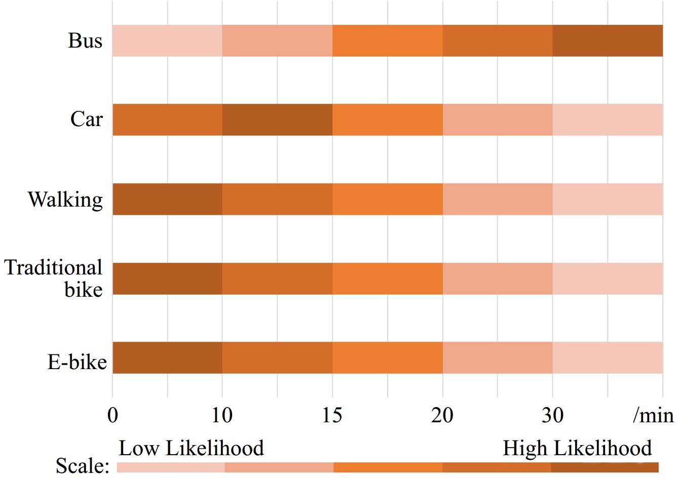
Figure 3.
The likelihood of using different transport modes for different travel times.
Naive Bayes classifier
-
This study also adopted the Naive Bayes classifier to investigate how different travel times influence the choice of transport mode, which could be used to compare the results from the multinomial logistic regression. Five Naive Bayes classifiers separately analysed samples travelled by bus, car, walking, traditional bike, and e-bike; the results output the probability of using the corresponding transport mode for different travel times, and other variables were regarded as independent variables. Each Naive Bayes classifier used a fivefold cross-validation procedure in Python via the Scikit-learn tool to obtain reliable modelling results. The relevant sample was randomly divided into five subsets, each containing 20% of the data. Four subsets (80% of the data) are the training set, and the remaining subset (20%) is the test set. Results have been summarised in Table 10.
Table 10. The probability of using different transport modes for different travel times via Naive Bayes.
Travel time (min) Probability Bus Car Walking Traditional bike E-bike ≤ 10 5.93% 10.32% 51.50% 29.38% 28.52% 10−15 8.05% 11.74% 21.28% 16.91% 18.73% 15−20 18.70% 24.07% 15.32% 24.26% 21.82% 20−30 40.51% 37.03% 9.75% 19.96% 23.45% > 30 26.81% 16.85% 2.15% 9.48% 7.48% Total 100.00% 100.00% 100.00% 100.00% 100.00% The values in boldface represent the highest probability of using the bus and car for different travel times. The output of multinomial logistic regression and the Naive Bayes classifier differ. To compare the performance of multinomial logistic regression and the Naive Bayes classifier, this study has compared the accuracy of these two models in predicting each mode choice (i.e., bus, car, walking, traditional bike, and e-bike), which is a method that has been commonly applied by existing studies[64,73,84]. As shown in Table 11, five Naive Bayes classifiers have higher prediction accuracy (0.37, 0.33, 0.59, 0.33, and 0.34) than multinomial logistic regression (0.22, 0.25, 0.20, 0.17, and 0.12) in predicting each mode choice. Also, by referring to Xiao et al.[77], and Yuan et al.[78], this study adopted DIC to compare these two types of models. As shown in Table 11, the DIC values from five Naive Bayes classifiers (226.43, 934.06, 512.49, 139.42, and 2,577.18) were much smaller than that of multinomial logistic regression (13,087.62). Therefore, the goodness-of-fit of Naive Bayes classifiers performs better. The following explanation concentrates on the results from the Naive Bayes classifiers.
Table 11. Comparison of the performance between multinomial logistic regression and Naive Bayes classifier.
Bus Car Walking Traditional
bikeE-bike Accuracy Naive Bayes classifiers 0.37 0.33 0.59 0.33 0.34 Multinomial logistic regression 0.22 0.25 0.20 0.17 0.12 DIC Naive Bayes classifiers 226.43 934.06 512.49 139.42 2,577.18 Multinomial logistic regression 13,087.62 According to the results summarised in Table 10 based on Naive Bayes classifiers, Table 12 and Fig. 4 shows that on the one hand, bus travellers and car travellers had similar probabilities of using the corresponding transport mode when travel time was between 15 and 30 min; on the other hand, bus travellers, and car travellers had relevantly higher probabilities of using the corresponding transport mode when travel time was between 15 and 30 min. Therefore, bus travel is possible to replace car travel when the travel time is between 15 and 30 min, which aligns with the findings from Liu et al.[9] that bus travel may have the potential to substitute for car travel when travel time is between 15 and 30 min. This is partly different from the results of the multinomial logistic regression, which presented that bus travel may potentially replace car travel when the travel time is between 15 and 20 min.
Table 12. The rank of the probability of using different transport modes for different travel times.
Travel time (min) Probability ranking Bus Car Walking Traditional bike E-bike 1 20 < x ≤ 30 20 < x ≤ 30 ≤ 10 ≤ 10 ≤ 10 2 > 30 15 < x ≤ 20 10 < x ≤ 15 15 < x ≤ 20 20 < x ≤ 30 3 15 < x ≤ 20 > 30 15 < x ≤ 20 20 < x ≤ 30 15 < x ≤ 20 4 10 < x ≤ 15 10 < x ≤ 15 20 < x ≤ 30 10 < x ≤ 15 10 < x ≤ 15 5 ≤ 10 ≤ 10 > 30 > 30 > 30 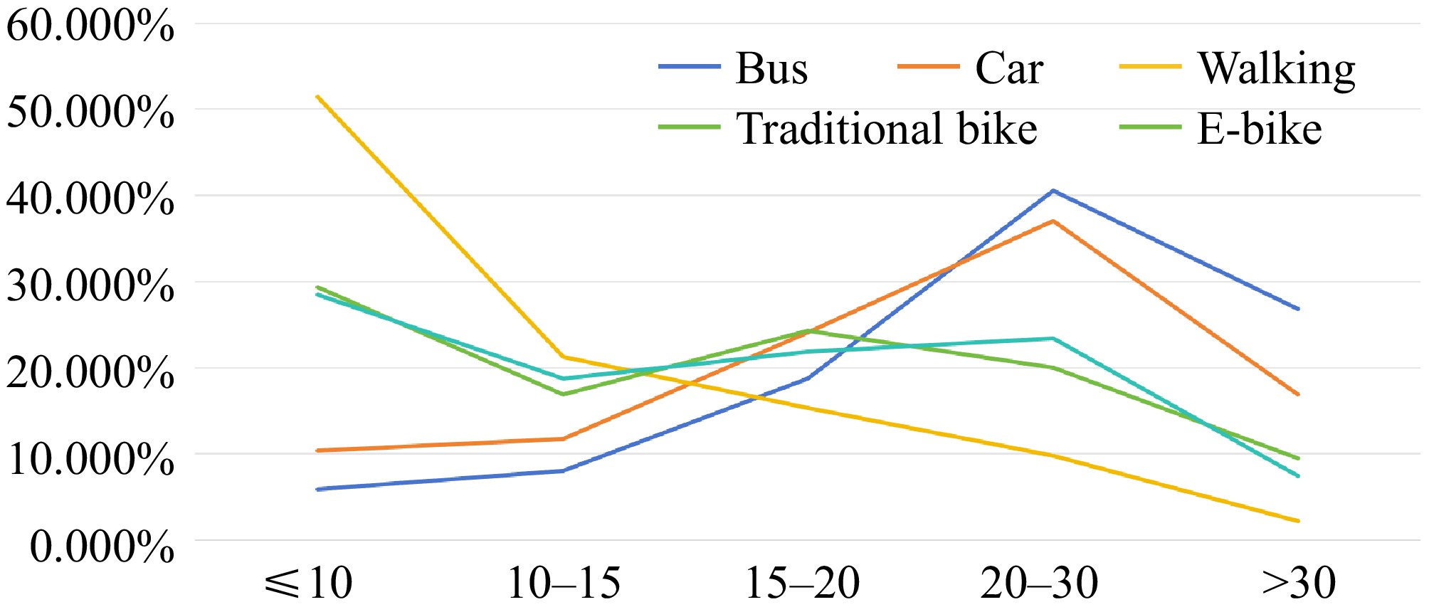
Figure 4.
The probability of using different transport modes for different travel times.
In addition, Fig. 4 also presents that traditional bike or e-bike travel may be possible to replace car travel when travel time is between 15 and 20 min; the potential may be higher than that of bus travel because of higher probabilities, which could be supplementary to the study by Liu et al.[9]. Although previous research has found that e-bikes have the potential to substitute for car usage and reduce ownership[85−91], few studies focused on the potential travel time for replacing car travel with e-bike travel.
-
This study introduced the background of the neglected Chinese third-tier cities and used data from the 2019 Yangzhou Residents' Travel Survey with 7,666 valid samples. Binary logistic regression was selected to investigate which factors could impact bus travel. Then, multinomial logistic regression and the Naive Bayes classifier were adopted to explore the potential of replacing car travel with bus travel. There are three key findings. First, this study examined the impact of socio-demographic and travel behaviour factors on daily bus use. Focused on socio-demographic characteristics, females, older adults, respondents with lower annual incomes, respondents who lived downtown, and respondents without cars were more likely to travel by bus. Focused on travel behaviour factors, respondents with less walking time to bus stops (≤ 5 min), less average waiting time for buses (≤ 10 min), travelling during the off-peak period, lower average number of trips per day, and longer travel time were more likely to travel by bus. Second, this study investigated the probabilities of people travelling by different travel modes (bus, car, walking, traditional bike, and e-bike) for different travel times. The goodness-of-fit of Naive Bayes classifiers performed better than that of multinomial logistic regression by comparing the models' accuracy and DIC. Third, according to the output of Naive Bayes classifiers, this study found that bus travel may potentially substitute for car travel when travel time is between 15 and 30 min.
There are two main contributions to this study. Empirically, this study focused on neglected Chinese third-tier cities, using Yangzhou as the case city, rather than Chinese prestigious cities (i.e., first-tier cities, new first-tier cities, or second-tier cities), which provide empirical evidence to enrich the current transport field. Theoretically, this study demonstrated that the Naive Bayesian classifier performs better than the multinomial logistic regression by comparing the models' accuracy and DIC. Through the Naive Bayesian classifier, this study indicated that bus travel may have the potential to replace car travel when travel time is between 15 and 30 min. This study also noted that traditional bike and e-bike travel may be possible to replace car travel when travel time is between 15 and 20 min via the Naive Bayesian classifier, which filled another research gap that existing studies have mainly considered the relationship between bus travel and car use and ignored the impacts of other transport modes[8].
In short, by exploring the probability of travelling by bus and other modes at different times, this study presented empirical evidence for the potential of bus travel to replace car travel, which could help reduce car use and relieve traffic congestion[9,12]. Correspondingly, this study drew relevant policy implications for improving bus transport in Chinese third-tier cities. First, females and older adults were more likely to use the bus[9,22,25,42,43]; thus, bus transport should focus on supplying more accessible facilities and services for them. Second, given that respondents with lower annual incomes were likely to travel by bus, it would be reasonable to offer discounted tickets to those who face financial constraints[9,12,18,26]. Third, since easier access to bus stops generally attracts more bus use[12,22], planners and policymakers should supply sufficient bus infrastructure in the non-central area, which could decrease walking time to bus stops. Fourth, to reduce waiting time and travel time for buses, on the one hand, bus transport should ensure punctuality and reliability[8,92]; on the other hand, increasing the frequency of public transport could decrease average waiting time[12,18,83]. Finally, besides prioritising the development of bus transport, planners and policymakers should implement other strategies for reducing car use and encourage residents to transfer car travel to bus travel, especially for medium- and long-distance journeys. Compared with more developed Chinese cities, third-tier cities usually only have one form of public transport: buses. Thus, planners and policymakers can consider these policy implications for broader regions, particularly cities with only buses as public transport.
Because of the characteristics of the adopted data in this study, the lack of heterogeneity analysis could be the main limitation of this study. On the one hand, although this study involved all age groups and considered whether respondents were employed or not, the sample was not classified by categories such as students, commuters, and retirees. Future studies could conduct deeper analysis to compare the results among students, commuters, and retirees on bus travel. On the other hand, since the secondary data did not clearly distinguish travel purposes between commuting and leisure, future studies could collect relevant information to compare and analyse the results for bus travel between commuting and leisure trips. Furthermore, since this study only adopted one secondary dataset based on one Chinese third-tier city, Yangzhou, more factors or variables than the dataset were not involved in the analysis. Thus, in the future, conducting surveys in different Chinese third-tier cities to collect more direct information related to bus travel (e.g., built environment and respondents' willingness to replace car travel with bus travel) can check the results of this study and widen the relevant policy implications to other ones. Although this study proved that the Naive Bayesian classifier has better accuracy and performance than multinomial logistic regression, existing empirical studies have compared broader machine learning methods in analysing travel mode choice, such as random forest[64,73], neural network[64,65,68], support vector machine[64,65,73], and extreme gradient boosting (XGBoost)[84]. Therefore, future studies could also involve these machine learning methods to explore bus travel in Chinese third-tier cities and compare their performance.
-
There are no animal or human subjects in this article, and informed consent is not applicable.
All the authors thank the financial support from the National Key R&D Program of China - Intergovernmental Cooperation in International Science and Technology Innovation (2024YFE0114400).
-
The authors confirm their contributions to the paper as follows: study conception and design: Liu Q, Liu Y, Xu X; data collection: Liu Q; analysis and interpretation of results: Liu Q, Liu Y, Xu X; draft manuscript preparation: Liu Q, Liu Y, Yin H, Xu X. All authors reviewed the results and approved the final version of the manuscript.
-
The datasets generated during and/or analyzed during the current study are available from the corresponding author upon reasonable request.
-
The authors declare that they have no conflict of interest.
- Supplementary File 1 Description of analysis methods.
- Supplementary Table S1 Results of the binary logistic regression (1 = travelled by bus, 0 = otherwise; n = 7,666).
- Copyright: © 2025 by the author(s). Published by Maximum Academic Press, Fayetteville, GA. This article is an open access article distributed under Creative Commons Attribution License (CC BY 4.0), visit https://creativecommons.org/licenses/by/4.0/.
-
About this article
Cite this article
Liu Q, Liu Y, Yin H, Xu X. 2025. Which factors impact bus travel, and the potential of replacing car travel with bus travel: an empirical study from a Chinese third-tier city. Digital Transportation and Safety 4(3): 195−206 doi: 10.48130/dts-0025-0018 

Which factors impact bus travel, and the potential of replacing car travel with bus travel: an empirical study from a Chinese third-tier city
- Received: 06 January 2025
- Revised: 07 April 2025
- Accepted: 09 May 2025
- Published online: 28 September 2025
Abstract: The role of transport in accelerating the development of Chinese cities has attracted widespread attention among global scholars. However, previous studies were primarily dominated by more prestigious Chinese first-tier, new first-tier, or second-tier cities rather than third-tier cities. It is worth noting that buses are usually the only form of public transport in Chinese third-tier cities; thus, prioritising the development of bus transport seems to play a vital role in these cities. This study introduced the background of the Chinese third-tier city and selected Yangzhou, a typical Chinese third-tier city, as the case area. The data were collected from the 2019 Yangzhou Residents' Travel Survey and binary logistic regression was considered to investigate which factors could impact bus travel. By comparing the multinomial logistic regression and the Naive Bayes classifier, the potential of replacing car travel with bus travel was verified. The results indicated that the Naive Bayesian classifier performs better, and bus travel may potentially replace car travel when travel time is between 15 and 30 min. Potential insights suggest policy implications for improving bus facilities and services.
-
Key words:
- Third-tier cities /
- Travel option /
- Binary logistic regression /
- Naive Bayes classifier