Integral of Sporopollenin Autofluorescence Intensity (ISAI), a novel marker for UV adaptation in spores/pollen

Xin-Lei Jia; Xi-Long Wang; Yi-Yun Chen; Li-Mi Mao; Hui Shen; Zhong-Nan Yang; Ying Xiao; Jing-Shi Xue; Xin-Lei Jia; Xi-Long Wang; Yi-Yun Chen; Li-Mi Mao; Hui Shen; Zhong-Nan Yang; Ying Xiao; Jing-Shi Xue

doi:10.48130/seedbio-0025-0016

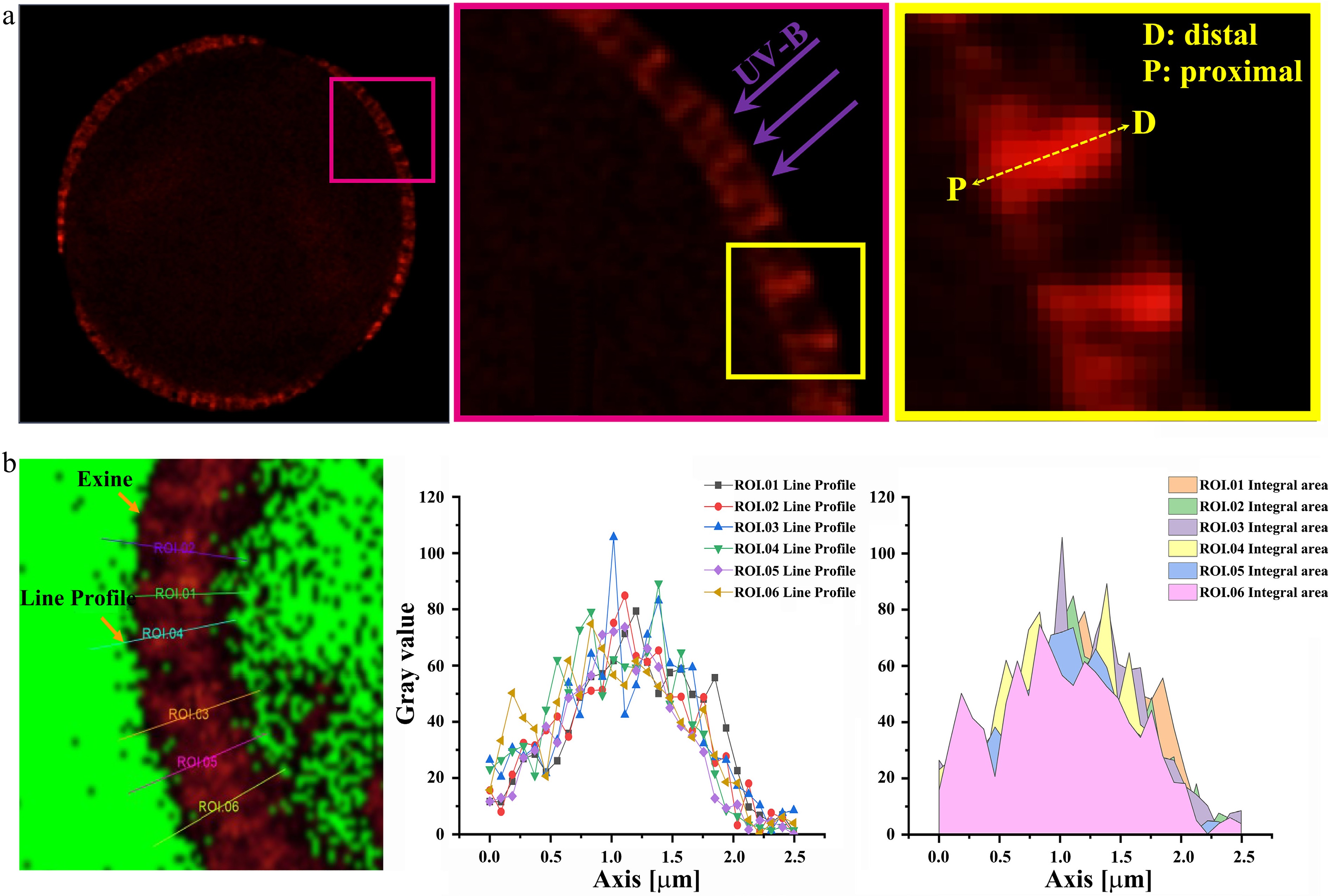
Figure 1.

The quantification of ISAI by using laser scanning confocal microscopy (LSCM). (a) The LSCM image of the maximum light section of spore/pollen wall in equatorial view. Left: the maximum light section of the spore/pollen in equatorial view. Middle: the magnified image of the pink box in the left image. UV-B damage the protoplasm only after they pass through the pollen wall. Right: the diagrammatic sketch of the distal-proximal axial of spore/pollen wall, and it is the magnified image of the yellow box in the middle image. UV-B damage the protoplasm only after they pass through the pollen wall along the distal-proximal axial. (D: distal; P: proximal). (b) Detection of autofluorescent intensity of the pollen by LSCM. ROI: region of interest. Left image: the diagram of the line profile of the pollen wall autofluorescence. The image is in the maximum light section of spore/pollen in the equatorial view. The signal intensity of exine was obtained using the line profile provided by LAS X (Leica) software. Middle image: line chart of the autofluorescent intensity of the pollen wall. Right image: the signal intensity of the pollen wall autofluorescent was obtained by using the method of integral area.

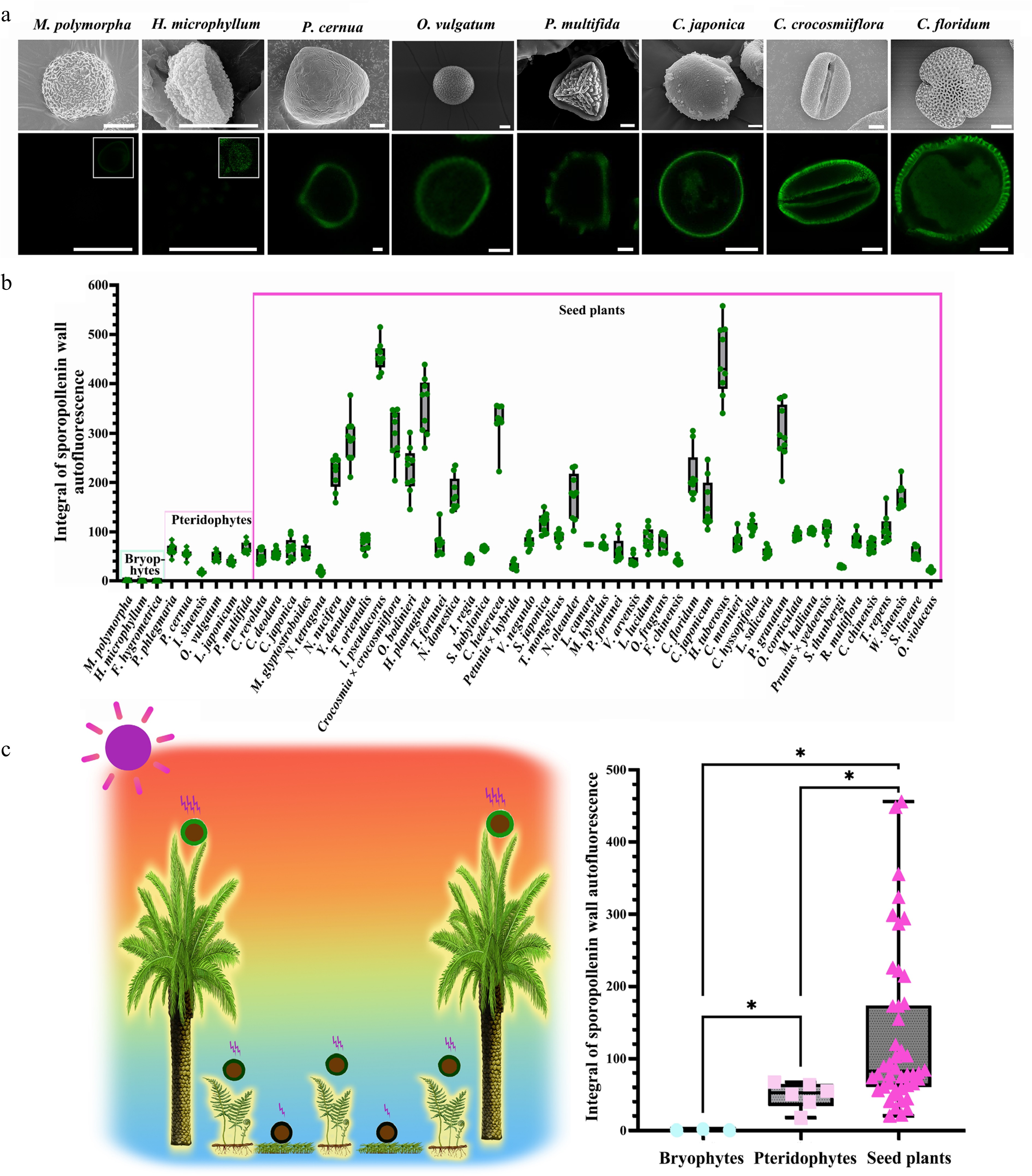
Figure 2.

ISAI varies among spores/pollen from distinct ecological niches. (a) Scanning electron microscope (SEM) and auto-fluorescence (Auto-flu) images of spore/pollen of several representative species. For SEM, scale bars = 10 μm; for LCSM, scale bars = 10 μm. For M. polymorpha and H. microphyllum, since the sporopollenin wall autofluorescence is very low, the picture with the image dynamic range adjusted is displayed in the upper right corner of the fluorescence picture. (b) Columnar diagram of spore/pollen wall autofluorescent intensity, 12 sites of each spore/pollen were selected for line profile, and nine spores or pollen grains were counted from each species. (mean ± SD, n = 9). (c) Statistical analysis of spore/pollen wall autofluorescent intensity. Left: summary of UV-B irradiation experienced by spores/pollen of land plants. Due to variations in the ecological niches of land plants and the spread distance of spores/pollen, the UV-B radiation experienced by spores/pollen in the terrestrial environment differ. Specifically, UV radiation intensities typically follow the order of seed plants > pteridophytes > bryophytes. Right: autofluorescent intensity of spore/pollen wall showed significant differences among bryophytes, pteridophytes, and seed plants (Mann-Whitney U test: Bryophytes vs Pteridophytes: Z = −2.19469, p = 1.19E-2; Bryophytes vs Seed plants: Z = −2.85665, p = 5.43E-5; Pteridophytes vs Seed plants: Z = −2.62071, p = 3.14E-3; *, p < 0.05).

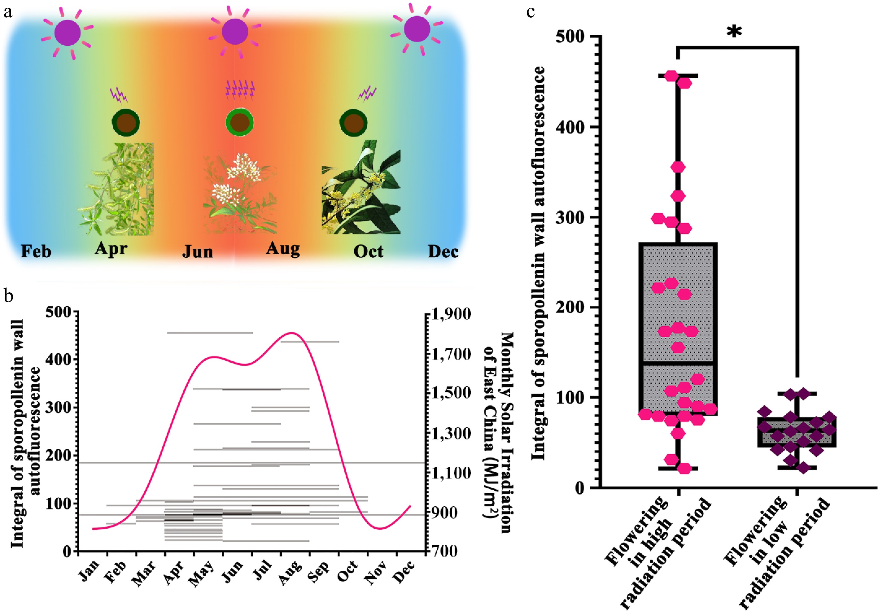
Figure 3.

Pollen ISAI of seed plants across different flowering periods. (a) Summary of UV-B irradiation experienced by the pollen of land plants in East China. East China's subtropical monsoon climate features intense UV radiation from June to August, during which flowering species may subject their pollen to increased solar irradiation. (b) Summary of florescence, integral of sporopollenin wall autofluorescence intensity, and the monthly solar irradiation of East China. The grey lines show the florescence and the integral of sporopollenin wall autofluorescence intensity of seed plants tested. The magenta line shows the variation of monthly solar irradiation of East China. The tested seed plants have different florescence and integral of sporopollenin wall autofluorescence intensity. (c) Statistical analysis of autofluorescent intensity of pollen wall of seed plants which flower under high and low radiation conditions. The pollen wall autofluorescence is significantly different between species which flowering in high radiation environment and low radiation environment (Mann-Whitney U test: Flowering in high radiation period vs Flowering in low radiation period: Z = −4.10761, p = 1.23E-5; *, p < 0.05).

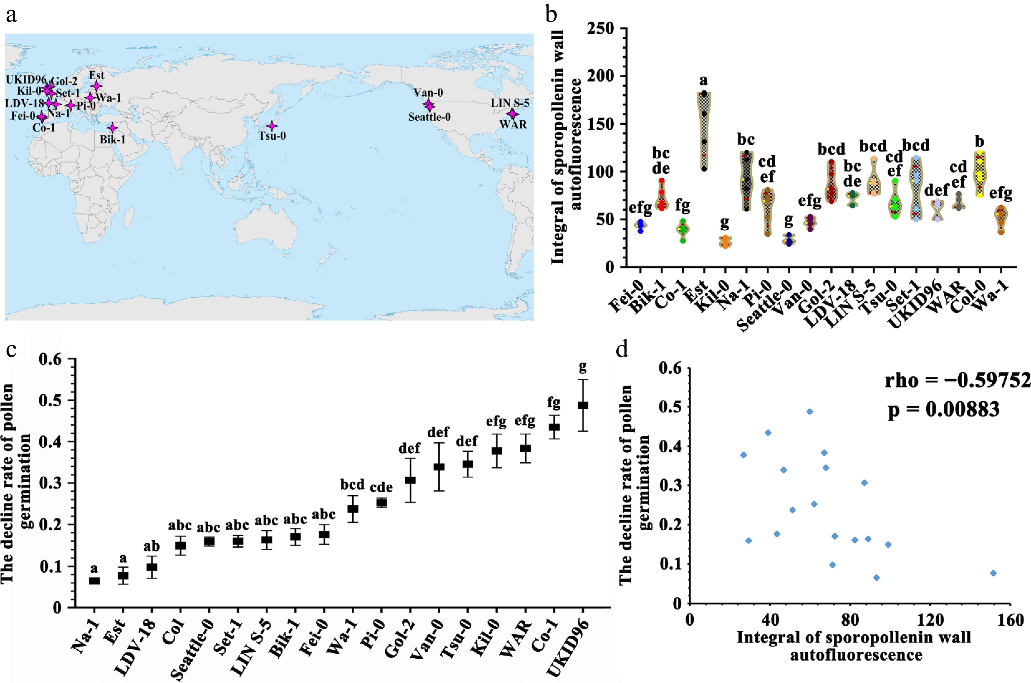
Figure 4.

The sporopollenin wall autofluorescence is correlated with UV-B defense ability of pollen grains in Arabidopsis thaliana ecotypes. (a) The geographical distribution of ecotypes used in this experiment. (b) Violin plot of the integral of sporopollenin wall autofluorescence intensity in A. thaliana ecotypes. The yellow line indicates the average value, the red line indicates the quartile value, and the data points are showed in the graph. Twelve measurement lines each pollen grain, five pollen grains each A. thaliana ecotype (mean ± SD, n = 5). Grouping information using the Tukey's Method and 95% confidence. Means that do not share a letter are significantly different. The A. thaliana ecotypes showed significant difference in the integral of sporopollenin wall autofluorescence. (c) Determination of pollen germination rate (mean ± SD, n = 4). Grouping information using Tukey's method and 95% confidence. Means that do not share a letter are significantly different. These A. thaliana ecotypes showed different decline rates under the UV-B treatment. (d) Spearman correlation analysis of the decline rates of pollen germination under the UV-B treatment in different A. thaliana ecotypes vs the integral of sporopollenin wall autofluorescence intensity (Spearman correlation: rho = −0.59752, p = 0.00883).