-
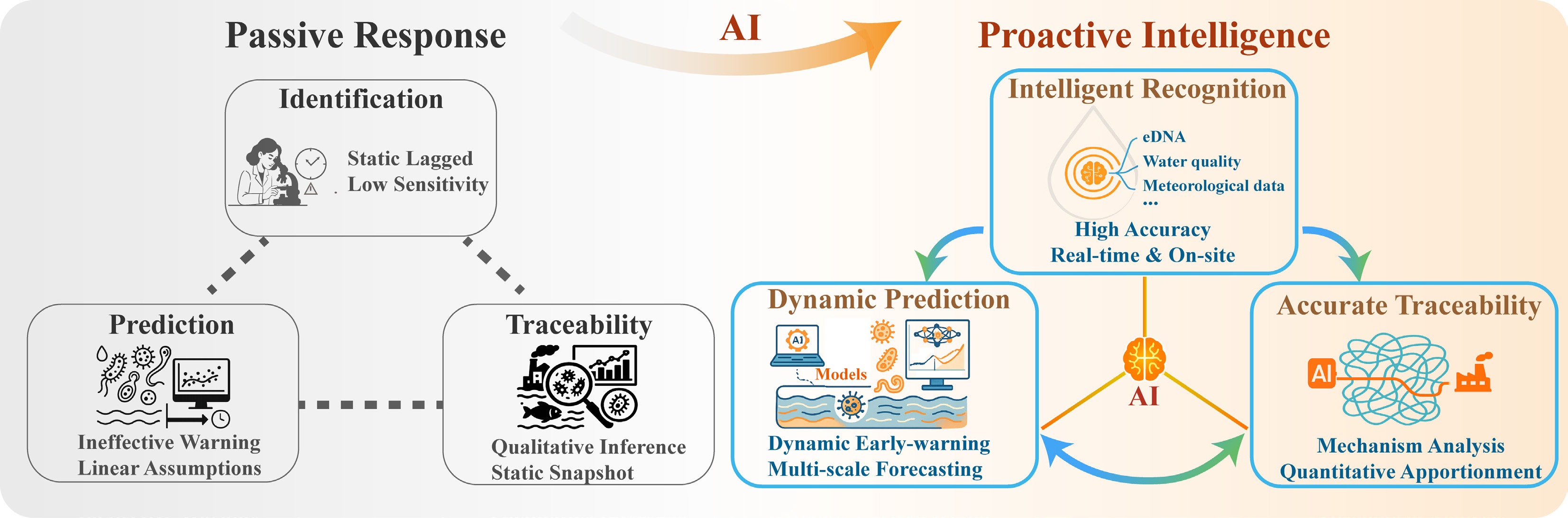
Figure 1.
Schematic illustration contrasting the traditional passive response paradigm (left) with the artificial intelligence (AI)-driven proactive intelligence framework (right) for managing biocontaminants in water environments. The passive approach is characterized by static identification with lagged detection and low sensitivity, prediction reliant on linear assumptions resulting in ineffective warnings, and traceability limited to qualitative inferences and snapshot analyses. In contrast, the AI-driven paradigm integrates intelligent identification using multi-source data (e.g., environmental DNA, water quality, and meteorological parameters) for real-time, high-accuracy monitoring; dynamic prediction models for early warning and multi-scale forecasting; and accurate traceability through mechanistic analysis and quantitative apportionment. This visual emphasizes the shift from disjointed, reactive methods to an integrated, data-driven system that enhances precision and responsiveness in pollution control.
-
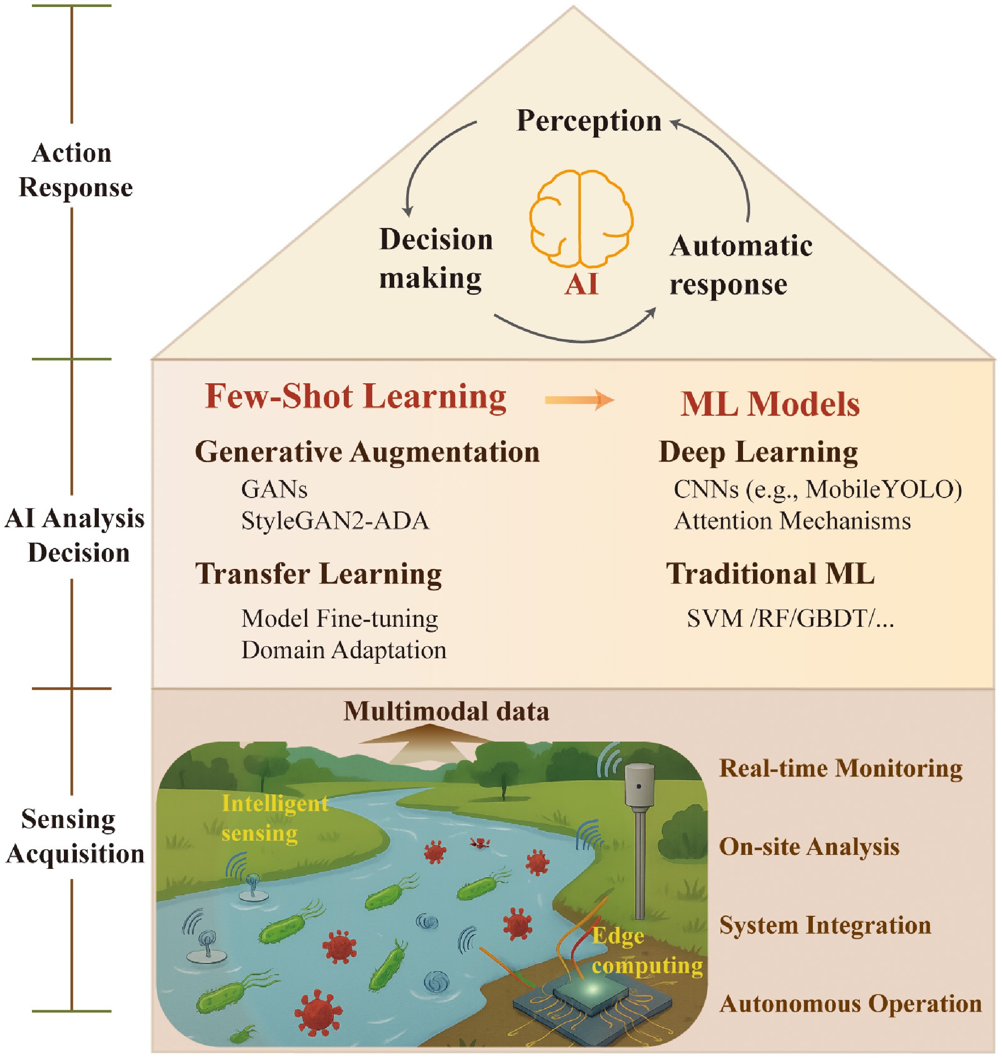
Figure 2.
Architectural framework of an AI-integrated intelligent perception and decision-making system for water environment management, depicted as a house-like structure to symbolize a holistic and stable infrastructure. The system features a hierarchical design with a central AI core that manages a closed loop of perception, decision-making, and automated response. This architecture is designed to ensure real-time interactivity and adaptive control. The middle layer integrates advanced machine learning approaches, including few-shot learning, to address data scarcity, and a diverse suite of models spanning deep learning and traditional algorithms for robust analysis. The base level illustrates the acquisition of multimodal data from intelligent sensing networks and edge computing devices, enabling capabilities such as real-time monitoring, on-site analysis, system integration, and autonomous operation. This visual underscores how AI synergizes data, models, and actions to evolve the biocontaminants management framework towards a dynamic, end-to-end intelligent system.
-
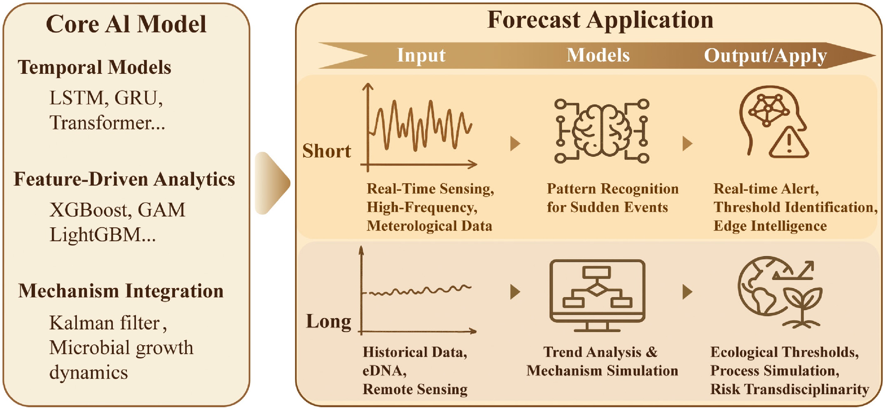
Figure 3.
A conceptual framework illustrating the integration of core AI models with multi-scale forecasting applications for water biocontaminants. The left panel (Core AI Model) categorizes foundational algorithmic approaches into three synergistic pillars: temporal models (e.g., LSTM, GRU, Transformer) for capturing dynamic patterns; feature-driven analytics (e.g., XGBoost, GAM) for identifying key influencing factors; and mechanism integration (e.g., Kalman filter, microbial growth dynamics) for incorporating domain knowledge. The right panel (Forecast Application) demonstrates how these models are deployed across temporal scales. Short-term forecasting uses real-time sensor and meteorological data, along with pattern recognition models, to generate immediate outputs such as alerts and edge intelligence. Long-term forecasting leverages historical, eDNA, and remote sensing data through trend analysis and mechanism simulation to predict ecological thresholds and enable transdisciplinary risk assessment. The schematic underscores the critical role of selecting and integrating appropriate AI architectures to allow precise, scalable predictions from operational warnings to strategic planning.
-
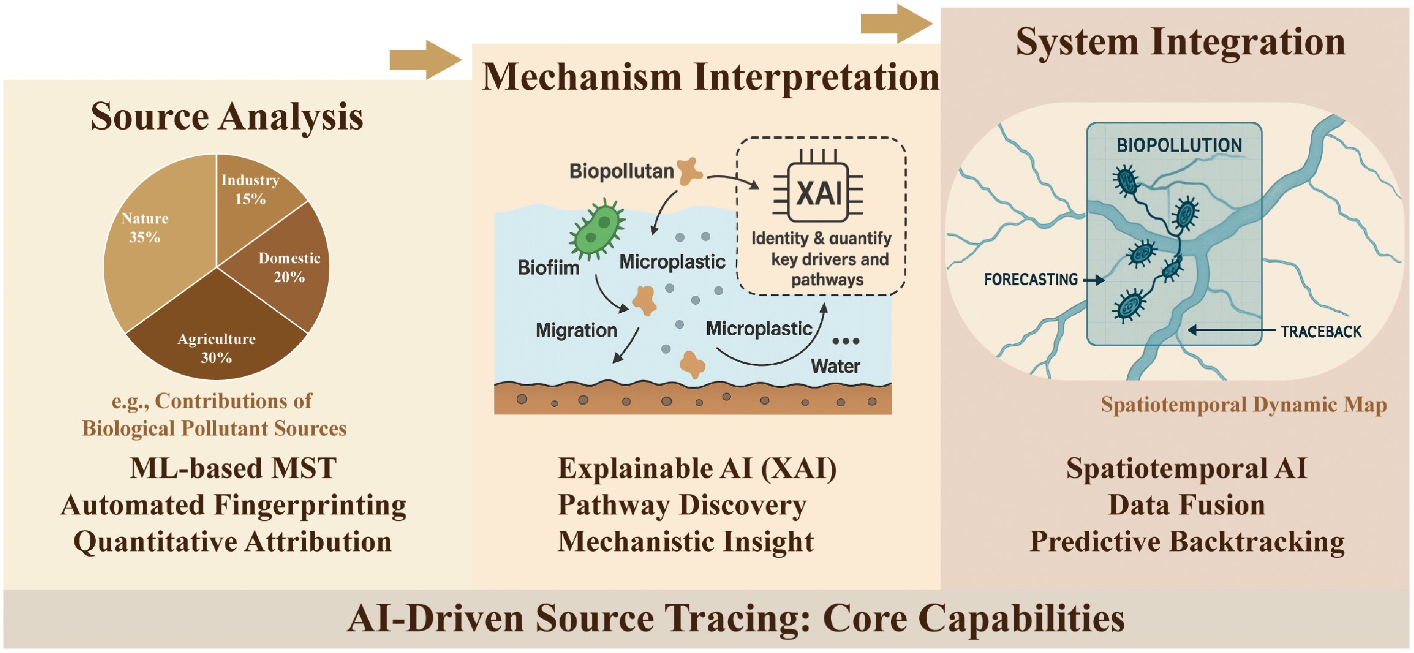
Figure 4.
A tripartite framework of AI-driven source tracing capabilities for biocontaminants in water environments. The framework progresses from source apportionment to mechanistic interpretation and culminates in spatiotemporal integration. The left panel (Source Analysis) demonstrates the application of ML-based MST for automated fingerprinting and quantitative attribution, as shown in a pie chart that decomposes the relative contributions of domestic, agricultural, industrial, and natural sources. The central panel (Mechanism Interpretation) highlights the role of XAI in identifying and quantifying key drivers and pathways, including interactions among microplastics, biofilms, and contaminants during migration, thereby uncovering causal mechanistic insights. The right panel (System Integration) illustrates the synthesis of these capabilities via spatiotemporal AI, which fuses multi-source data to create a dynamic map enabling predictive backtracking of contamination events and forecasting of their dispersal. Collectively, this figure demonstrates how AI transforms source tracing from a static, descriptive exercise into a dynamic, interpretable, and predictive system essential for proactive risk management.
-
Biocontaminants Detection category Data type AI model Key performance Timeliness Ref. Harmful algal bloom eDNA, remote sensing,
water quality parametersMultimodal (sequence, image, numerical) Gradient boosting decision tree (GBDT) MAPE = 11.20% Laboratory [53] Water quality data Numerical/tabular Supervised ML Accuracy = 98.09% Real-time [54] Microscopy images Image CNN, CNN-SVM Accuracy = 99.66% Laboratory [44] Pathogens Optical sensors Spectral CNN Accuracy ≥ 95% Real-time [55] Signal/spectral Naive bayes (NB), decision tree (DT) Accuracy ≥ 95% Real-time [56] Image SVM, random forest (RF), ANN, extreme gradient boosting (XGBoost) Accuracy ≈ 99.9% Real-time [57] Fluorescence sensors Spectral K-nearest neighbors (KNN), principal component analysis (PCA) Accuracy = 100% Real-time [58] Raman spectroscopy Spectral CNN Accuracy = 98% Laboratory [59] Electrochemical aptasensor Numerical/tabular GAM, ridge, partial least squares (PLS), GBDT RMSE = 0.19 Real-time [60] Electrochemical sensors Numerical/tabular Multilayer perceptron (MLP), gradient boosting (GB), RF Accuracy = 97% Real-time [61] Parasites Microbial, water quality, meteorological parameters Multimodal RF, XGBoost Accuracy =
80.3% (Crypto),
82.6% (Giardia)Laboratory [62] Microscopy images Image YOLOv4 Accuracy = 100% Laboratory [63] Image DenseNet, ResNet Accuracy = 100% Laboratory [64] ARGs Metagenomics Sequence RF AUC ≈ 0.99 Laboratory [65] qPCR Numerical DT R2 = 0.87 Laboratory [66] Table 1.
Landscape of AI-driven detection technologies for aquatic biocontaminants
-
Biocontaminants AI model Best key performance Prediction horizon Ref. Harmful algal bloom CNN NSE = 0.84 3, 7 d [77] General RNN, SVM R2 ≈ 0.82 1, 2 weeks [78] ANN, SVM R2 ≈ 0.97 7 d [79] CNN R2 ≈ 0.93 1 week [80] ANN Accuracy = 89% 1 month [81] LSTM R2 ≈ 0.821 3 months [82] MLP R2 = 0.26 1 week [83] Support vector regression (SVR), MLP, RF R2 = 0.78 1 d [84] GBM Accuracy ≈ 90% 10 d [85] GBDT R2 = 0.97 1, 2 week [86] ANN, SVM Accuracy = 81% 1 week [87] ANN and SVM Accuracy = 100% 1 week [88] Pathogens RF Accuracy = 97% Summer months [89] ANN, RF Accuracy = 81% Several hours [90] LASSO, RF R2 = 0.62 1 d [91] Boosted regression trees (BRT) R2 = 0.67 1–2 weeks [92] Viruses PLS, XGBoost, categorical boosting, GRU, LSTM R2 = 0.97 Several hours [73] ANN, MLP R2 = 0.89 Several hours [93] Table 2.
Prediction horizon of AI models for aquatic biocontaminant outbreaks
Figures
(4)
Tables
(2)